This post is in relation to the part 4. of a multipart ML/DL forecast post series on Australian flight patronage by route, pre-covid. Approaches used are:
GluonTS
DeepAR
N-BEATS
All parts of series:
1. Some pre analysis (basic EDA analysis is not covered as already included in previous posts)
2. ‘Sequence’ style models - ARIMA etc
3. ML style models - XGBoost etc including nesting and ensembling
4. Deep learning models (GLuonTS etc)
5. Summary of conclusions
2 Load Libraries
Code
#| echo: false# Time Series MLlibrary(tidymodels)library(modeltime)library(modeltime.gluonts)library(modeltime.ensemble)# Corelibrary(tidyverse)library(lubridate)library(timetk)# Timing & Parallel Processinglibrary(tictoc)library(future)library(doFuture)library(here)library(skimr)library(gt)library(here)
3 Load Data
Loading pre-prepared data as well as some parameters. Also setting up parallel processing.
GluonTS is a Python package for probabilistic time series modeling, focusing on deep learning based models, based on PyTorch and MXNet. It was developed by Amazon.
Some quotes from the GluonTS website are useful:
” In forecasting, there is the implicit assumption that observable behaviours of the past that impact time series values continue into the future. ”
” Naturally, it’s impossible to forecast the unpredictable. For instance, in 2019 it was virtually impossible to account for the possibility of travel restrictions due to the Covid-19 pandemic when trying to forecacst travel demand for 2020.
Thus, forecasting operates on the caveat that the underlying factors that generate the time series values don’t fundamentally change in the future. It is a tool to predict the ordinary and not the surprising.”
In this analysis we get around this ’problem, by only predicting passenger numbers up to the beginning of covid effect, and maybe soon post covid impact.
Another key aspect of GluonTS is that it is probabilistic - predicting distributions of outcomes not just one value per time point. This is very useful.
Another useful feature of GluonTS is that it includes the concept of Global models which enables many time series to be trained together and then used to make probabilistic predictions for each time series. In this analysis we have 70 or so time series - one for each route.
GluonTS makes many models available in Python. A number of the models and concepts (eg hierarchical forecasting are based/wrapped on the Forecast package in R and the related textbook Forecasting: Principles and Practice.
This analysis uses the modeltime.gluonts package in R to interface to GluonTS. This R library enables an R interface to some of the GluonTS models. The following analysis uses:
# A tibble: 4 × 4
  variable        type      role      source
  <chr>           <list>    <chr>     <chr>
1 route           <chr [3]> predictor original
2 date            <chr [1]> predictor original
3 rowid           <chr [2]> indicator original
4 passenger_trips <chr [2]> outcome   original
6.1 DeepAR
DeepAR was also developed by Amazon (as part of Sagemaker) which is particularly suited to cross-sectional analysis (eg routes), in that the time series are trained jointly across all routes (in our case).
A few different combinations of epoch numbers and batch sizes per epoch have been tried
Modeltime.gluonts package allows for 2 types of implementations: Standard or Ensemble. The following models include a mix of both, also with varying hyper-parameters.
N-BEATS Model Specification (regression)

Main Arguments:
  id = route
  freq = M
  prediction_length = FORECAST_HORIZON
  lookback_length = c(FORECAST_HORIZON, 2 * FORECAST_HORIZON)
  loss_function = MASE
  bagging_size = 2
  epochs = 5
  num_batches_per_epoch = 35

Computational engine: gluonts_nbeats_ensemble
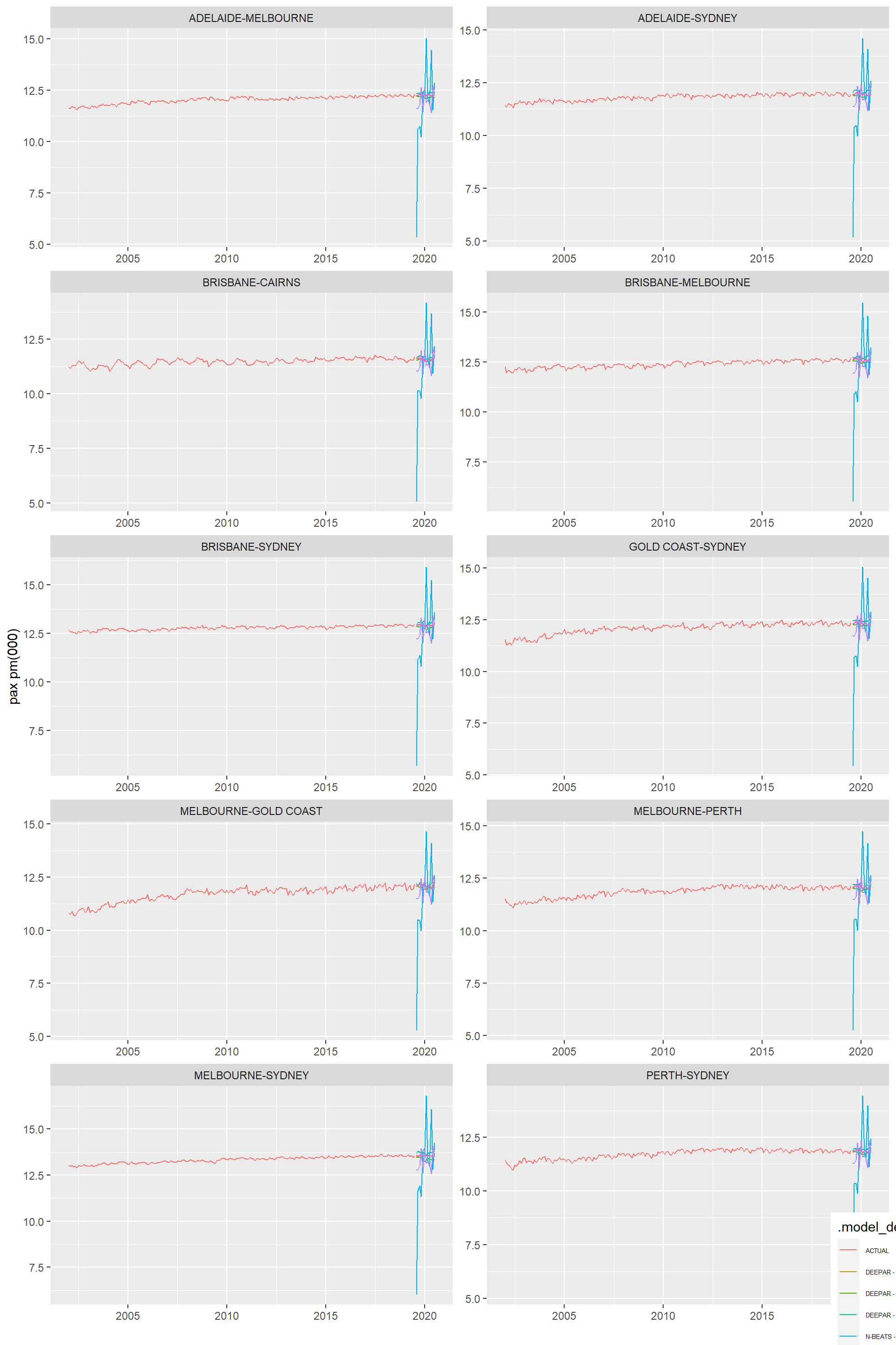
7 Modeltime Comparison
The following code puts all models in the one table, renames them and produces an accuracy report, sorted by ‘MAAPE’, best at top. Unfortunately it does not want to render in quarto.
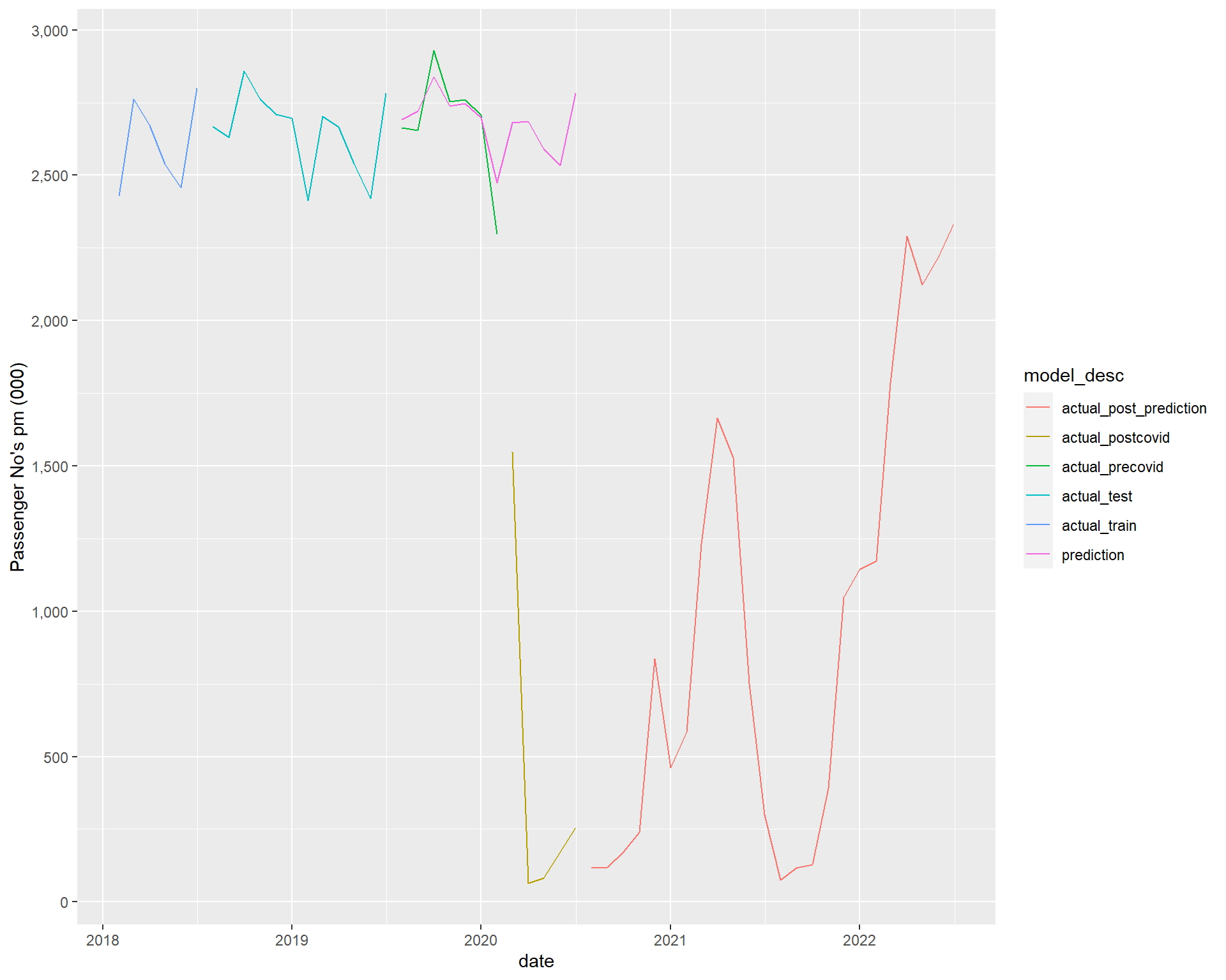
So not too bad for predictions precovid (ie before the cliff), which is our focus.
Source Code
---title: "Flight Forecasting with Deep Learning - Incomplete"author: "Stephen J Parton"date: "2022-12-27"categories: [code, analytics, flights, forecasting]website: sidebar: style: "docked" search: trueformat: html: theme: literatoc: truetoc-title: Contentsnumber-sections: truenumber-depth: 3code-fold: showcode-summary: "Code"code-tools: trueexecute: echo: true warning: false error: falsefreeze: truecache: true---## IntroductionThis post is in relation to the part 4. of a multipart ML/DL forecast post series on Australian flight patronage by route, pre-covid. Approaches used are:- GluonTS - DeepAR - N-BEATSAll parts of series:1\. Some pre analysis (basic EDA analysis is not covered as already included in previous posts)2\. 'Sequence' style models - ARIMA etc3\. ML style models - XGBoost etc including nesting and ensembling4\. Deep learning models (GLuonTS etc)5\. Summary of conclusions## Load Libraries```{r, libraries}#| echo: false# Time Series MLlibrary(tidymodels)library(modeltime)library(modeltime.gluonts)library(modeltime.ensemble)# Corelibrary(tidyverse)library(lubridate)library(timetk)# Timing & Parallel Processinglibrary(tictoc)library(future)library(doFuture)library(here)library(skimr)library(gt)library(here)```## Load DataLoading pre-prepared data as well as some parameters. Also setting up parallel processing.```{r, data}top_routes_prep_df <-read_rds(here("./posts/aust_domestic_flights/artifacts/top_routes_prep_df.rds"))start <-"2001-01-01"end <-"2019-07-01"horizon_nested <-12end_precovid <-dmy("01-02-2020")top_x <-10#d2 <- dmy("01-07-2022")max_act <-max(top_routes_prep_df$date)max_test <-ymd(end)max_pred <- max_test %m+%months(horizon_nested)FORECAST_HORIZON <-1*12lag_period <-1*12rolling_periods <-c(3,6,12)# * Parallel Processing ----registerDoFuture()n_cores <- parallel::detectCores()plan(strategy = cluster,workers = parallel::makeCluster(n_cores))```## PreprocessingSome additional wrangling.```{r, wrangle}# topx listtopx <- top_routes_prep_df %>%group_by(route) %>%summarise(passenger_trips =sum(passenger_trips)) %>%ungroup() %>%slice_max(passenger_trips, n=top_x) %>%arrange(desc(passenger_trips)) %>%select(route) %>%pull() %>%as.character()full_data_tbl <- top_routes_prep_df %>%group_by(route) %>%#initial wrangleselect(route,date,passenger_trips) %>%mutate(route =as.character(route)) %>%group_by(route) %>%summarise_by_time(date, .by ="month", passenger_trips =sum(passenger_trips)) %>%pad_by_time( date,.by ="month",.pad_value =0,.start_date =min(top_routes_prep_df$date)) %>%filter_by_time(.date_var = date,.start_date = start, .end_date = end ) %>%ungroup()full_data_tbl <- full_data_tbl %>%tk_augment_timeseries_signature() %>%select(-c(day:mday7)) %>%select(-contains(".iso"),-contains(".xts"))full_data_tbl <- full_data_tbl %>%#log transform targetmutate(passenger_trips =log1p(passenger_trips),index.num =log1p(index.num),diff =log1p(diff),year =log1p(year)) %>%#groupwise manipulationgroup_by(route) %>%future_frame(.date_var = date,.length_out = FORECAST_HORIZON,.bind_data =TRUE ) %>%# Fouriertk_augment_fourier(.date_var = date,.periods =c(0.5* FORECAST_HORIZON, FORECAST_HORIZON),.K =1 ) %>%# Lagstk_augment_lags(.value = passenger_trips,.lags = FORECAST_HORIZON ) %>%# Rolling Featurestk_augment_slidify(.value = passenger_trips_lag12,.f =~mean(.x,na.rm =TRUE),.period =c(6, FORECAST_HORIZON, 2* FORECAST_HORIZON),.partial =TRUE,.align ='center' ) %>%ungroup() %>%rowid_to_column(var ="rowid")data_prepared_tbl <- full_data_tbl %>%filter(!is.na(passenger_trips)) %>%drop_na()future_tbl <- full_data_tbl %>%filter(is.na(passenger_trips)) route_prep_validation <- top_routes_prep_df %>%# filter(route %in% topx ) %>% filter(date > max_test ) %>%ungroup() %>%mutate(passenger_trips =log1p(passenger_trips)) %>%group_by(route)```## Split DataSplit into training and testing sets.### Training Set (top 10 routes)```{r, split,fig.width=10,fig.height=15}splits <- data_prepared_tbl %>%time_series_split(date_var = date,assess = FORECAST_HORIZON,cumulative =TRUE )training(splits) %>%group_by(route) %>%filter(route %in% topx) %>%plot_time_series( date, passenger_trips,.facet_ncol =2,.smooth =FALSE,.title ="Training Splits" )max_train <-max(training(splits)$date)```### Testing Set (top 10 routes)```{r, testing,fig.width=10,fig.height=15}testing(splits) %>%group_by(route) %>%filter(route %in% topx) %>%plot_time_series( date, passenger_trips,.facet_ncol =2,.smooth =FALSE,.title ="Testing Splits" )```## GLUONTS[GluonTS](https://ts.gluon.ai/stable/) is a Python package for probabilistic time series modeling, focusing on deep learning based models, based on [PyTorch](https://pytorch.org/) and [MXNet](https://mxnet.apache.org/). It was developed by Amazon.Some quotes from the GluonTS website are useful:" In forecasting, there is the implicit assumption that observable behaviours of the past that impact time series values continue into the future. "" Naturally, it's impossible to forecast the unpredictable. For instance, in 2019 it was virtually impossible to account for the possibility of travel restrictions due to the Covid-19 pandemic when trying to forecacst travel demand for 2020.Thus, forecasting operates on the caveat that the underlying factors that generate the time series values don't fundamentally change in the future. It is a tool to predict the ordinary and not the surprising."In this analysis we get around this 'problem, by only predicting passenger numbers up to the beginning of covid effect, and maybe soon post covid impact.Another key aspect of GluonTS is that it is probabilistic - predicting distributions of outcomes not just one value per time point. This is very useful.Another useful feature of GluonTS is that it includes the concept of Global models which enables many time series to be trained together and then used to make probabilistic predictions for each time series. In this analysis we have 70 or so time series - one for each route.GluonTS makes [many models](https://ts.gluon.ai/stable/getting_started/models.html) available in Python. A number of the models and concepts (eg hierarchical forecasting are based/wrapped on the Forecast package in R and the related textbook [Forecasting: Principles and Practice](https://otexts.com/fpp3/hts.html).This analysis uses the modeltime.gluonts package in R to interface to GluonTS. This R library enables an R interface to some of the GluonTS models. The following analysis uses:- DeepAR- N-Beats```{r,gluon_recipe}# 3.0 GLUONTS MODELS ----# * GLUON Recipe Specification ----#Gluon only needs Target,ID(groups) and daterecipe_spec_gluon <-recipe( passenger_trips ~ route + date + rowid,data =training(splits)) %>%update_role(rowid,new_role ="indicator")#recipe_spec_gluon %>% prep() %>% juice()recipe_spec_gluon %>%prep() %>%summary()```### DeepARDeepAR was also developed by Amazon (as part of Sagemaker) which is particularly suited to cross-sectional analysis (eg routes), in that the time series are trained jointly across all routes (in our case).A few different combinations of epoch numbers and batch sizes per epoch have been tried#### DeepAR Model 1 - epochs 5; batch size/ epoch:50```{r,deepar_1}model_spec_1_deepar <-deep_ar(#Required paramsid ="route",freq ="M",prediction_length = FORECAST_HORIZON,#trainerepochs =5,#DeepAR specificcell_type ="lstm") %>%set_engine("gluonts_deepar")#wflowwflw_fit_deepar_1 <-workflow() %>%add_model(model_spec_1_deepar) %>%add_recipe(recipe_spec_gluon) %>%fit(training(splits))model_spec_1_deepar```#### DeepAR Model 2 - epochs 10; batch size/ epoch: 35 ```{r,deepar_2}# Model 2: Increase Epochs, Adjust Num Batches per Epoch#model specmodel_spec_2_deepar <-deep_ar(id ="route",freq ="M",prediction_length = FORECAST_HORIZON,epochs =10,num_batches_per_epoch =35,#DeepAR specificcell_type ="lstm") %>%set_engine("gluonts_deepar")#wflowwflw_fit_deepar_2 <-workflow() %>%add_model(model_spec_2_deepar) %>%add_recipe(recipe_spec_gluon) %>%fit(training(splits))model_spec_2_deepar```#### DeepAR Model 3 - epochs 10; batch size/ epoch: 50 ```{r,deepar_3}# Model 3: Increase Epochs, Adjust Num Batches Per Epoch, & Add Scalingmodel_spec_3_deepar <-deep_ar(id ="route",freq ="M",prediction_length = FORECAST_HORIZON,epochs =10,num_batches_per_epoch =50,scale =TRUE,#DeepAR specificcell_type ="lstm") %>%set_engine("gluonts_deepar")#wflowwflw_fit_deepar_3 <-workflow() %>%add_model(model_spec_3_deepar) %>%add_recipe(recipe_spec_gluon) %>%fit(training(splits))model_spec_3_deepar```### N-Beats (Neural Basis Expansion Analysis for Time Series)N-BEATS is [a type of neural network that was first described in a 2019 article by Oreshkin et al](https://arxiv.org/abs/1905.10437)Modeltime.gluonts package allows for 2 types of implementations: Standard or Ensemble. The following models include a mix of both, also with varying hyper-parameters.#### N-Beats Model 4 - Default (epochs:5)```{r,nbeats_4}# * N-BEATS Estimator ----# Model 4: N-BEATS defaultmodel_spec_nbeats_4 <-nbeats(id ="route",freq ="M",prediction_length = FORECAST_HORIZON,lookback_length =2* FORECAST_HORIZON) %>%set_engine("gluonts_nbeats")wflw_fit_nbeats_4 <-workflow() %>%add_model(model_spec_nbeats_4) %>%add_recipe(recipe_spec_gluon) %>%fit(training(splits))model_spec_nbeats_4```#### N-Beats Model 5 - Default (epochs:5;loss fn:MASE)```{r, nbeats_5}# Model 5: N-BEATS, loss function:MASE, Reduce Epochs 2model_spec_nbeats_5 <-nbeats(id ="route",freq ="M",prediction_length = FORECAST_HORIZON,lookback_length =2* FORECAST_HORIZON,epochs =5,loss_function ="MASE") %>%set_engine("gluonts_nbeats")wflw_fit_nbeats_5 <-workflow() %>%add_model(model_spec_nbeats_5) %>%add_recipe(recipe_spec_gluon) %>%fit(training(splits))model_spec_nbeats_5```#### N-Beats Model 6 - Default (ensemble; epochs:5; loss fn:MASE)```{r, nbeats_6}# Model 6: N-BEATS, Model 5 ensemblemodel_spec_nbeats_6 <-nbeats(id ="route",freq ="M",prediction_length = FORECAST_HORIZON,lookback_length =c(FORECAST_HORIZON, 2* FORECAST_HORIZON),epochs =5,num_batches_per_epoch =35,loss_function ="MASE",bagging_size =2) %>%set_engine("gluonts_nbeats_ensemble")wflw_fit_nbeats_6 <-workflow() %>%add_model(model_spec_nbeats_6) %>%add_recipe(recipe_spec_gluon) %>%fit(training(splits))model_spec_nbeats_6```## Modeltime ComparisonThe following code puts all models in the one table, renames them and produces an accuracy report, sorted by 'MAAPE', best at top. Unfortunately it does not want to render in quarto.```{r,accuracy}#modeltime_calibrate()# Modeltime Comparison ----model_tbl_submodels <-modeltime_table( wflw_fit_deepar_1, wflw_fit_deepar_2, wflw_fit_deepar_3,# wflw_fit_nbeats_4, wflw_fit_nbeats_5, wflw_fit_nbeats_6)model_tbl_submodels <- model_tbl_submodels %>%update_model_description(1,"DEEPAR - unscaled, 5ep") %>%update_model_description(2,"DEEPAR - unscaled, 10ep") %>%update_model_description(3,"DEEPAR - scaled, 10ep") %>%update_model_description(4,"N-BEATS - 5ep") %>%update_model_description(5,"N-BEATS - 5ep,MASE") %>%update_model_description(6,"N-BEATS - ens, 5ep,MASE") # model_tbl_submodels_calibrate <- model_tbl_submodels %>% # modeltime_calibrate(new_data = testing(splits))# # # # Forecast Accuracy - not rendering????# model_tbl_submodels_calibrate %>%# modeltime_accuracy(# #testing(splits),# metric_set = extended_forecast_accuracy_metric_set()) %>%# arrange(maape) %>%# gt::gt() %>%# gt::fmt_number(# columns = 4:10,# decimals = 3)```## Refit ModelsModels are then refit to full train/test data.```{r, refit}submodels_refitted_tbl <- model_tbl_submodels %>%modeltime_refit(data_prepared_tbl)submodels_refitted_tbl```## Make Predictions```{r, prediction_all}submodels_pred_ <- submodels_refitted_tbl %>%modeltime_forecast(new_data = future_tbl,actual_data = data_prepared_tbl,keep_data =TRUE)head(submodels_pred_)``````{r, calibrate}``````{r, pred_graph,fig.width=10,fig.height=15}submodels_pred_ %>%filter(route %in% topx) %>%group_by(route) %>%ggplot(aes(x = .index, y = .value,colour = .model_desc))+geom_line() +scale_y_continuous(labels = comma) +labs(x ="", y ="pax pm(000)") +facet_wrap(~ route, ncol=2, scales ="free") +theme(legend.position =c(1,0)) +theme(legend.text =element_text(size=5))# plot_modeltime_forecast(# .trelliscope = F,# .facet_ncol = 2,# .title = "Predictions - Top10 Routes"# )```The accuracy stats and graph suggest that some of these are not so good. ..## Ensemble ModelEnsemble the top deep learning models:- Model 6 - N-Beats ensuite- Model 3 - DeepAR scaled, 10 epochs- Model 2 - DeepAR unscaled 10 epochsThere is no reason not to also include some ML models in the ensemble - we will do that in a separate post.```{r, ensemble}# Modeltime Comparison ----model_tbl_ensemble <-modeltime_table(#wflw_fit_deepar_1, wflw_fit_deepar_2, wflw_fit_deepar_3,##wflw_fit_nbeats_4,#wflw_fit_nbeats_5, wflw_fit_nbeats_6)model_tbl_ensemble <- model_tbl_ensemble %>%#update_model_description(1,"DEEPAR - unscaled, 5ep") %>% update_model_description(1,"DEEPAR - unscaled, 10ep") %>%update_model_description(2,"DEEPAR - scaled, 10ep") %>%#update_model_description(4,"N-BEATS - 5ep") %>% #update_model_description(5,"N-BEATS - 5ep,MASE") %>% update_model_description(3,"N-BEATS - ens, 5ep,MASE") model_tbl_ensemble_wtd <- model_tbl_ensemble %>%ensemble_weighted(loadings =c(1,3,4)) %>%modeltime_table()# model_tbl_ensemble_calibrate <- model_tbl_ensemble_wtd %>% # modeltime_calibrate(new_data = testing(splits),# id = "route")# # # model_tbl_ensemble_calibrate %>% # # summarize_accuracy_metrics(# # truth = actual,# # estimate = forecast,# # metric_set = extended_forecast_accuracy_metric_set()# # ) %>% arrange(smape)# # # model_tbl_ensemble_calibrate %>%# modeltime_accuracy(# #testing(splits),# metric_set = extended_forecast_accuracy_metric_set()# ) %>%# arrange(rmse) %>%# gt::gt() %>%# gt::fmt_number(# columns = 4:10,# decimals = 3)```## Refit Ensemble to Full Train/Test Data Set and Graph```{r,refit_ensemble}model_tbl_ensemble_refit <- model_tbl_ensemble_wtd %>%# model_tbl_ensemble_calibrate %>% modeltime_refit(data_prepared_tbl)model_tbl_ensemble_pred <- model_tbl_ensemble_refit %>%modeltime_forecast(new_data = future_tbl,actual_data = data_prepared_tbl,keep_data =TRUE,conf_by_id =TRUE ) ``````{r}model_tbl_ensemble_pred_data <- model_tbl_ensemble_pred %>%select(model_id = .model_id,model_desc = .model_desc,act_pred = .key, date, route, .value,) %>%bind_rows(route_prep_validation %>%mutate(model_desc ="ACTUAL_VALIDN") %>%select(route,date,model_desc,.value = passenger_trips) ) %>%filter(route %in% topx, date>lubridate::ymd("2018-01,01")) %>%mutate(pax_nos_000 =expm1(.value)/1000) %>%group_by(route)# model_tbl_ensemble_pred_data_wide <- model_tbl_ensemble_pred_data %>% # select(route,date,model_desc,pax_nos_000) %>% # group_by(route,date,model_desc) %>% # pivot_wider(# names_from = model_desc,values_from = pax_nos_000# ) %>% # arrange(route,date)g_data <- model_tbl_ensemble_pred_data %>%select(date,route,model_desc,pax_nos_000) %>%group_by(route,date,model_desc) %>%summarise(pax_nos_000=sum(pax_nos_000, na.rm =TRUE)) %>%mutate(model_desc =case_when( model_desc =="ENSEMBLE (WEIGHTED): 3 MODELS"~"prediction", date <= max_train ~"actual_train", date <= max_test ~"actual_test", date <= end_precovid ~"actual_precovid", date <= max_pred ~"actual_postcovid",TRUE~"actual_post_prediction" )) %>%arrange(route,date)g <- g_data %>%ggplot(aes(x = date, y = pax_nos_000,group = route,colour = model_desc )) +geom_line() +# geom_ribbon(aes(ymin = conf_lo,# ymax = conf_hi,# color = model_desc),# alpha = 0.2) +scale_y_continuous(labels = comma) +labs(x ="", y ="pax pm(000)") +facet_wrap(vars(route), ncol =2, scales ="free")+theme(legend.position =c(1,0)) +theme(legend.text =element_text(size=9))#gplotly::ggplotly(g)```## Aggregated Prediction - All routes```{r,graph, fig.width=10,fig.height=8}g_data_acc <- g_data %>%select(date,model_desc,pax_nos_000) %>%group_by(date,model_desc) %>%summarise(pax_nos_000 =sum(pax_nos_000,na.rm =TRUE)) %>%# select(-c(model_id,.index,.key)) %>% # pivot_longer(# cols = !date,# names_to = "actual_prediction",# values_to = "pax_nos_000"# ) %>% mutate(pax_nos_000 =ifelse(pax_nos_000 ==0, NA,pax_nos_000))g1 <- g_data_acc %>%ggplot(aes(x=date, y=pax_nos_000, colour = model_desc ))+geom_line() +# geom_ribbon(aes(ymin = conf_lo,# ymax = conf_hi,# color = model_desc),# alpha = 0.2) +scale_y_continuous("Passenger No's pm (000)",breaks = scales::breaks_extended(8),labels = scales::label_comma() )g1```So not too bad for predictions precovid (ie before the cliff), which is our focus.```{r}#| echo: falsefeature_engineering_artifacts_list_gluon <-list(#datadata =list(data_prepared_tbl = data_prepared_tbl,future_tbl = future_tbl ),#recipesrecipes =list(recipe_spec_gluon = recipe_spec_gluon ),#models/workflowsmodels =list(wflw_fit_deepar_1 = wflw_fit_deepar_1,wflw_fit_deepar_2 = wflw_fit_deepar_2,wflw_fit_deepar_3 = wflw_fit_deepar_3,wflw_fit_nbeats_4 = wflw_fit_nbeats_4,wflw_fit_nbeats_5 = wflw_fit_nbeats_5,wflw_fit_nbeats_6 = wflw_fit_nbeats_6,model_tbl_ensemble = model_tbl_ensemble ))# feature_engineering_artifacts_list_gluon# feature_engineering_artifacts_list_gluon %>% # write_rds(here("./posts/aust_domestic_flights/artifacts/feature_engineering_artifacts_list_gluon.rds"))```