Code
library(tidymodels)
library(modeltime.h2o)
library(tidyverse)
library(timetk)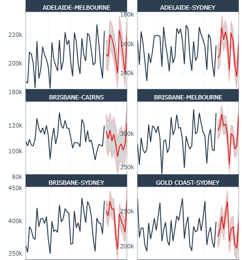
This analysis is one section of a multi-part set of posts looking at forecasting on domestic Australian flight volumes by route in the period prior to when covid largely shut the industry down. Its intention is just to provide me with examples over the main models to save time on future projects.It is split into:
Some pre analysis (basic EDA analysis is not covered as already included in previous posts)
‘Sequence’ style models - ARIMA etc
ML style models - XGBoost etc including nesting and ensembling
Deep learning models (GLuonTS etc)
Summary of conclusions
This post is in relation to the part 4 - focussing on H20, usimg the modeltime package to connect. This post is actually using ML models, but will be expanded to include deep learning approaches
it uses the modeltime H20 documentation
library(tidymodels)
library(modeltime.h2o)
library(tidyverse)
library(timetk)All data is loaded, except Brisbane-Emerald route is excluded as it caused problems, probably due to lack of data.
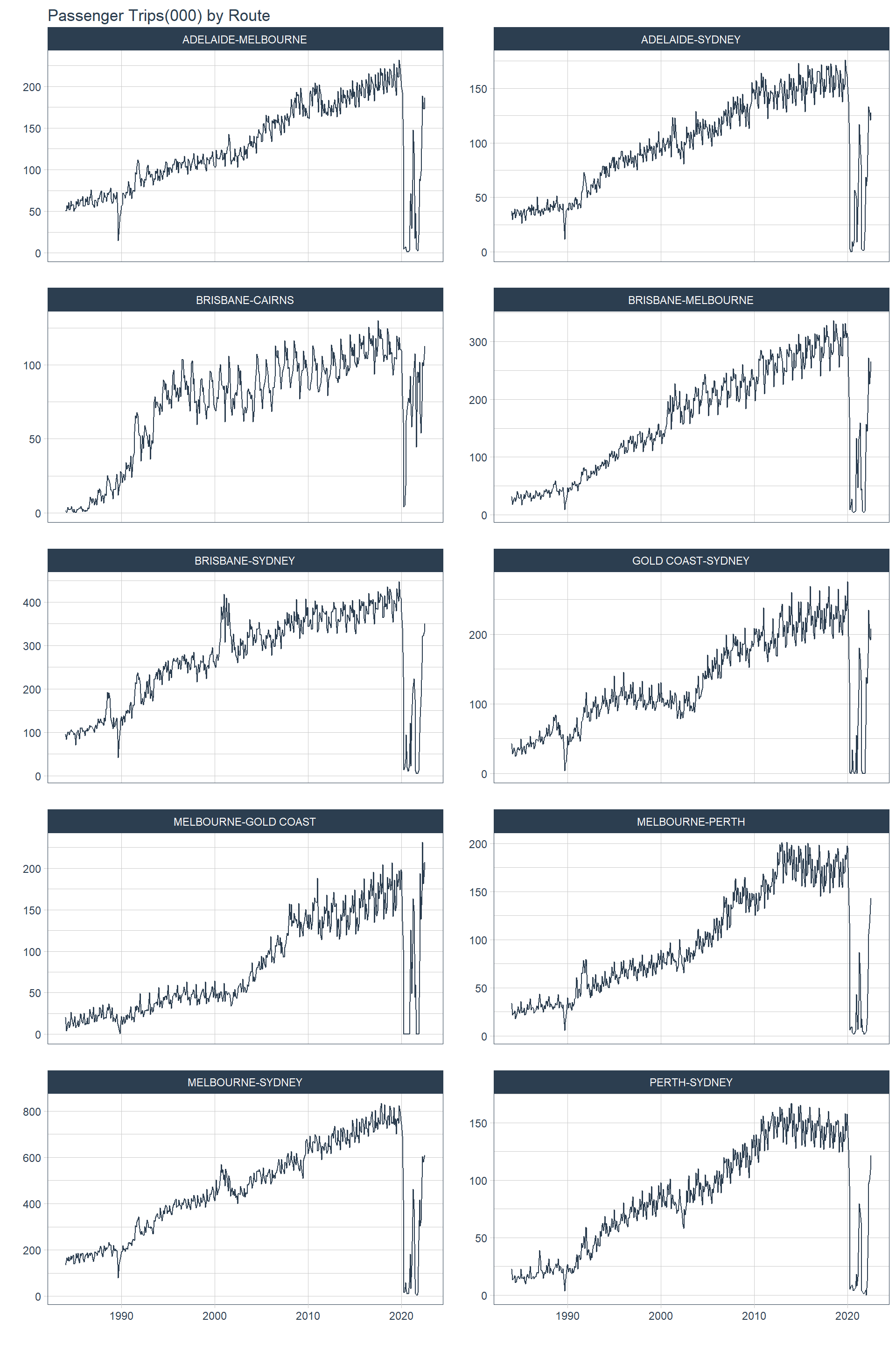
The top 10 routes are shown in order of overall patronage
top_x   <- 10
start   <- "2001-01-01"
end     <- "2019-07-01"
horizon <-  "1 year"

top_routes_prep_df <- read_rds("./artifacts/top_routes_prep_df.rds") %>%
  filter(route != "BRISBANE-EMERALD") %>% #dodgy for some reason
  #rowid_to_column(var = "id") %>%
  select(date,route,passenger_trips)

topx <- top_routes_prep_df %>%
  group_by(route) %>%
  summarise(passenger_trips = sum(passenger_trips)) %>%
  ungroup() %>%
  slice_max(passenger_trips, n=top_x) %>%
  arrange(desc(passenger_trips)) %>%
  select(route) %>%
  pull() %>%
  as.character()

topx %>% knitr::kable()| x |
|---|
| MELBOURNE-SYDNEY |
| BRISBANE-SYDNEY |
| BRISBANE-MELBOURNE |
| GOLD COAST-SYDNEY |
| ADELAIDE-MELBOURNE |
| ADELAIDE-SYDNEY |
| MELBOURNE-PERTH |
| PERTH-SYDNEY |
| MELBOURNE-GOLD COAST |
| BRISBANE-CAIRNS |
These graphs include full history. Covid period will be excluded for future analysis (bit hard to predict that little black swan).
top_routes_prep_df %>%
  filter(route %in% topx) %>%
  group_by(route) %>%
  plot_time_series(
    .date_var    = date,
    .value       = passenger_trips/1000,
    .facet_ncol  = 2,
    .smooth      = F,
    .interactive = F,
    .title       = "Passenger Trips(000) by Route"
  )
Data filtered to targetted period and then is split into trainig and test sets. Test set is 12 months.
data_tbl <- top_routes_prep_df %>%
  filter(date %>% between_time(start,end))


splits <- time_series_split(data_tbl, assess = horizon, cumulative = TRUE)

recipe_spec <- recipe(passenger_trips ~ ., data = training(splits)) %>%
    step_timeseries_signature(date)

train_tbl <- training(splits) %>% bake(prep(recipe_spec), .)
test_tbl  <- testing(splits)  %>% bake(prep(recipe_spec), .)

#min(test_tbl$date)
splits
<Analysis/Assess/Total>
<12751/828/13579># Initialize H2O
h2o.init(
nthreads = -1,
ip = 'localhost',
port = 54321
) Connection successful!
R is connected to the H2O cluster:
H2O cluster uptime: 2 hours 52 minutes
H2O cluster timezone: Australia/Brisbane
H2O data parsing timezone: UTC
H2O cluster version: 3.38.0.3
H2O cluster version age: 1 month and 7 days
H2O cluster name: H2O_started_from_R_spinb_yru550
H2O cluster total nodes: 1
H2O cluster total memory: 3.75 GB
H2O cluster total cores: 8
H2O cluster allowed cores: 8
H2O cluster healthy: TRUE
H2O Connection ip: localhost
H2O Connection port: 54321
H2O Connection proxy: NA
H2O Internal Security: FALSE
R Version: R version 4.2.2 (2022-10-31 ucrt) # Optional - Set H2O No Progress to remove progress bars
h2o.no_progress()model_spec <- automl_reg(mode = 'regression') %>%
set_engine(
engine = 'h2o',
max_runtime_secs = 60*60,
max_runtime_secs_per_model = 60,
max_models = 10,
nfolds = 5,
#exclude_algos = c("DeepLearning"),
verbosity = NULL,
seed = 786
)
model_specH2O AutoML Model Specification (regression)
Engine-Specific Arguments:
max_runtime_secs = 60 * 60
max_runtime_secs_per_model = 60
max_models = 10
nfolds = 5
verbosity = NULL
seed = 786
Computational engine: h2o model_fitted <- model_spec %>%
fit(passenger_trips ~ ., data = train_tbl) model_id rmse mse
1 StackedEnsemble_AllModels_1_AutoML_4_20221230_153853 4623.464 21376415
2 StackedEnsemble_BestOfFamily_1_AutoML_4_20221230_153853 4736.108 22430716
3 GBM_5_AutoML_4_20221230_153853 4738.926 22457424
4 GBM_3_AutoML_4_20221230_153853 5017.286 25173157
5 GBM_4_AutoML_4_20221230_153853 5085.078 25858014
6 GBM_1_AutoML_4_20221230_153853 5603.475 31398934
mae rmsle mean_residual_deviance
1 2625.410 NaN 21376415
2 2789.898 NaN 22430716
3 2787.829 NaN 22457424
4 2800.649 NaN 25173157
5 2843.318 NaN 25858014
6 2889.674 NaN 31398934
[12 rows x 6 columns] model_fitted parsnip model object
H2O AutoML - Stackedensemble
--------
Model: Model Details:
==============
H2ORegressionModel: stackedensemble
Model ID: StackedEnsemble_AllModels_1_AutoML_4_20221230_153853
Number of Base Models: 10
Base Models (count by algorithm type):
deeplearning drf gbm glm
1 2 6 1
Metalearner:
Metalearner algorithm: glm
Metalearner cross-validation fold assignment:
Fold assignment scheme: AUTO
Number of folds: 5
Fold column: NULL
Metalearner hyperparameters:
H2ORegressionMetrics: stackedensemble
** Reported on training data. **
MSE: 3217224
RMSE: 1793.662
MAE: 1164.881
RMSLE: NaN
Mean Residual Deviance : 3217224
H2ORegressionMetrics: stackedensemble
** Reported on cross-validation data. **
** 5-fold cross-validation on training data (Metrics computed for combined holdout predictions) **
MSE: 21376415
RMSE: 4623.464
MAE: 2625.41
RMSLE: NaN
Mean Residual Deviance : 21376415
Cross-Validation Metrics Summary:
mean sd
mae 2620.668000 54.265266
mean_residual_deviance 21332104.000000 1110405.600000
mse 21332104.000000 1110405.600000
null_deviance 24041516000000.000000 1477628900000.000000
r2 0.997734 0.000133
residual_deviance 54455750000.000000 4141945600.000000
rmse 4617.392000 121.426810
rmsle NA 0.000000
cv_1_valid cv_2_valid
mae 2665.413000 2617.336000
mean_residual_deviance 22474568.000000 21760620.000000
mse 22474568.000000 21760620.000000
null_deviance 24430357000000.000000 22966381000000.000000
r2 0.997614 0.997571
residual_deviance 58299027000.000000 55772467000.000000
rmse 4740.735000 4664.828000
rmsle NA NA
cv_3_valid cv_4_valid
mae 2647.775100 2644.215000
mean_residual_deviance 21071190.000000 21798888.000000
mse 21071190.000000 21798888.000000
null_deviance 25562297000000.000000 25167888000000.000000
r2 0.997853 0.997777
residual_deviance 54869380000.000000 55935947000.000000
rmse 4590.336400 4668.927700
rmsle NA NA
cv_5_valid
mae 2528.600600
mean_residual_deviance 19555256.000000
mse 19555256.000000
null_deviance 22080662000000.000000
r2 0.997853
residual_deviance 47401940000.000000
rmse 4422.132300
rmsle NAleaderboard_tbl <- automl_leaderboard(model_fitted)
leaderboard_tbl %>% knitr::kable()| model_id | rmse | mse | mae | rmsle | mean_residual_deviance |
|---|---|---|---|---|---|
| StackedEnsemble_AllModels_1_AutoML_4_20221230_153853 | 4623.464 | 21376415 | 2625.410 | NA | 21376415 |
| StackedEnsemble_BestOfFamily_1_AutoML_4_20221230_153853 | 4736.108 | 22430716 | 2789.898 | NA | 22430716 |
| GBM_5_AutoML_4_20221230_153853 | 4738.926 | 22457424 | 2787.829 | NA | 22457424 |
| GBM_3_AutoML_4_20221230_153853 | 5017.286 | 25173157 | 2800.649 | NA | 25173157 |
| GBM_4_AutoML_4_20221230_153853 | 5085.078 | 25858014 | 2843.318 | NA | 25858014 |
| GBM_1_AutoML_4_20221230_153853 | 5603.475 | 31398934 | 2889.674 | NA | 31398934 |
| GBM_2_AutoML_4_20221230_153853 | 5633.260 | 31733613 | 2944.514 | NA | 31733613 |
| GBM_grid_1_AutoML_4_20221230_153853_model_1 | 6170.972 | 38080898 | 3323.607 | NA | 38080898 |
| DeepLearning_1_AutoML_4_20221230_153853 | 15622.131 | 244050990 | 11268.303 | NA | 244050990 |
| DRF_1_AutoML_4_20221230_153853 | 23504.606 | 552466523 | 12546.398 | 2.691383 | 552466523 |
| XRT_1_AutoML_4_20221230_153853 | 82152.863 | 6749092971 | 48764.480 | 3.175682 | 6749092971 |
| GLM_1_AutoML_4_20221230_153853 | 97131.095 | 9434449699 | 56375.288 | 3.267512 | 9434449699 |
So AutoML and stacked ensembles thereof lead the way, deep learning approaches not really ranking!
Now,
modeltime_tbl <- modeltime_table(
    model_fitted
)

modeltime_tbl
# Modeltime Table
# A tibble: 1 × 3
.model_id .model .model_desc
<int> <list> <chr>
1 1 <fit[+]> H2O AUTOML - STACKEDENSEMBLEcalibration_tbl <- modeltime_tbl %>%
modeltime_calibrate(
new_data = test_tbl,
id = "route")
forecast_test_tbl <- calibration_tbl %>%
modeltime_forecast(
new_data = test_tbl,
actual_data = data_tbl,
keep_data = TRUE,
conf_by_id = T
) %>%
group_by(route)
#calibration_tblUsing the top model in the leaderboard- Auto_ML Stacked Ensemble
forecast_test_tbl %>%
  filter(route %in% topx,
         lubridate::year(date)> 2015) %>%
    plot_modeltime_forecast(
        .facet_ncol = 2,
        .interactive = T,
        .title = "Forecast v Test Data - top 10 Routes"
    )
So forecasts look pretty good…
Another look at accuracy measures of top model only.
calibration_tbl %>%
  modeltime_accuracy(metric_set = extended_forecast_accuracy_metric_set()) %>%
knitr::kable()| .model_id | .model_desc | .type | mae | mape | maape | mase | smape | rmse | rsq |
|---|---|---|---|---|---|---|---|---|---|
| 1 | H2O AUTOML - STACKEDENSEMBLE | Test | 2277.27 | Inf | 15.97232 | 0.02854 | 19.08186 | 3768.153 | 0.9988767 |
Before doing any predictions, we need to refit model to full dataset (train and test), so that prediction is based on most recent data!
data_prepared_tbl <- bind_rows(train_tbl, test_tbl)

future_tbl <- data_prepared_tbl %>%
    group_by(route) %>%
    future_frame(.date_var   = date,
                 .length_out = "1 year") %>%
    ungroup()

future_prepared_tbl <- bake(prep(recipe_spec), future_tbl)

refit_tbl <- calibration_tbl %>%
    modeltime_refit(data_prepared_tbl)
model_id rmse mse
1 StackedEnsemble_AllModels_1_AutoML_5_20221230_154413 4478.597 20057827
2 StackedEnsemble_BestOfFamily_1_AutoML_5_20221230_154413 4653.480 21654877
3 GBM_5_AutoML_5_20221230_154413 4663.906 21752021
4 GBM_3_AutoML_5_20221230_154413 4874.181 23757643
5 GBM_4_AutoML_5_20221230_154413 5018.797 25188324
6 GBM_1_AutoML_5_20221230_154413 5148.774 26509875
mae rmsle mean_residual_deviance
1 2525.244 NaN 20057827
2 2708.357 NaN 21654877
3 2704.795 NaN 21752021
4 2737.018 NaN 23757643
5 2806.473 NaN 25188324
6 2758.185 NaN 26509875
[12 rows x 6 columns] prediction <- refit_tbl %>%
modeltime_forecast(
new_data = future_prepared_tbl,
actual_data = data_prepared_tbl,
keep_data = TRUE,
conf_by_id = T
) %>%
group_by(route)
prediction %>%
filter(route %in% topx,
lubridate::year(date)> 2015) %>%
plot_modeltime_forecast(
.facet_ncol = 2,
.interactive = T,
.title = "Passenger Trip Prediction - top 10 Routes"
)I could compare the above prediction to the actuals, and i did on the base analyses, but it is a bit pointless due to the covid cliff, which is not in the analysis. Might include it as/if data is updated and some normality resumes.
model_fitted %>%
  save_h2o_model(path = "./artifacts/h20_model1", overwrite = TRUE)

#model_h2o <- load_h2o_model(path = "./artifacts/h20_model1")

#h2o.shutdown(prompt = FALSE)