Notes to Myself - Flight Forecast with ML Nested models

1 Introduction

This file runs a nested forecasting approach on top Australian domestic routes (70 or so) prior to covid. This is just an exploratory exercise and remains a work in progress.

This analysis uses ML Models as follows

Auto ARIMA
XGBoost
Prophet Boost
Random Forest
SVM
Neural Net
MARS
THIEF

Only XGBoost/ Prophet Boost have been tuned (based on Syd-Melb route only and using the same hyper-parameters as appropriate).

The forecast period is 12 months from end of testing, which is July 2019, so missing the Covid dive, which is still shown.

This will all look better in a Shiny app, coming soon…

2 Load Packages

Tidyverse, Tidymodels, Modeltime, parallel processing etc.

3 Load Data

Data has largely been pre-processed, and is loaded from rds files.

Code

#here()
top_routes_prep_df <- read_rds(here("./posts/aust_domestic_flights/artifacts/top_routes_prep_df.rds"))

start          <- "2001-01-01"
end            <- "2019-07-01"
horizon_nested <- 12
end_precovid <- dmy("01-02-2020")
#d2 <- dmy("01-07-2022")
max_act   <- max(top_routes_prep_df$date)
max_test  <- ymd(end)
max_pred  <- max_test %m+% months(horizon_nested)


filter_r       <- "N"
city           <- "BRISBANE"
top_x          <- 10

# * Parallel Processing ----
registerDoFuture()
n_cores <- parallel::detectCores()
plan(
  strategy = cluster,
  workers  = parallel::makeCluster(n_cores)
)

4 Wrangling

Some initial wrangling

Code

route_prep <- top_routes_prep_df %>%
  select(route,date,passenger_trips) %>%
  group_by(route) %>%
  summarise_by_time(date, .by = "month", passenger_trips = sum(passenger_trips)) %>%
  pad_by_time(date, .by       = "month",.pad_value = 0)


topx <- top_routes_prep_df %>% 
  group_by(route) %>% 
  summarise(passenger_trips = sum(passenger_trips)) %>% 
  ungroup() %>% 
  slice_max(passenger_trips, n=top_x) %>% 
  arrange(desc(passenger_trips)) %>% 
  select(route) %>% 
  pull() %>% 
  as.character()

route_prep_raw <- route_prep %>%
  filter(route %in% topx ) %>% 
  filter_by_time(.date_var    = date,.start_date = start, .end_date = end ) %>%
  ungroup() %>%
  mutate(passenger_trips      = log1p(passenger_trips)) %>%
  group_by(route)

route_prep_validation <- route_prep %>%
  filter(route %in% topx ) %>% 
  filter(date > max_test ) %>%
  ungroup() %>%
  mutate(passenger_trips      = log1p(passenger_trips)) %>%
  group_by(route)


# * Nested Time Series ----
route_prep_nested <- route_prep_raw %>%
  extend_timeseries(
    .id_var        = route,
    .date_var      = date,
    .length_future = horizon_nested

  ) %>%
  tk_augment_fourier(date,.periods = c(3,6,12)) %>%
  tk_augment_lags(passenger_trips, .lags = 12) %>%
  tk_augment_slidify(
    passenger_trips_lag12,
     .f       = ~mean(.x,na.rm = T),
     .period  = c(.25 * 12,.5 * 12, 12),
     .partial = T,
     .align   = "center"
  ) %>%

  nest_timeseries(
    .id_var        = route,
    .length_future = horizon_nested
  ) %>%
  split_nested_timeseries(
    .length_test   = horizon_nested
  ) %>%
  ungroup()
  #rowid_to_column(var = "rowid")

route_prep_nested_train <- extract_nested_train_split(route_prep_nested)
route_prep_nested_test  <- extract_nested_test_split(route_prep_nested)



max_train <- max(route_prep_nested_train$date)

Top Routes, ordered in descending order (of passengers numbers over total review period) :

Code

topx %>% kable()

x
MELBOURNE-SYDNEY
BRISBANE-SYDNEY
BRISBANE-MELBOURNE
GOLD COAST-SYDNEY
ADELAIDE-MELBOURNE
ADELAIDE-SYDNEY
MELBOURNE-PERTH
PERTH-SYDNEY
MELBOURNE-GOLD COAST
BRISBANE-CAIRNS

5 Recipes

3 Recipes have been established:

Base Recipe
Auto Arima Recipe
Tunable XG Boost Recipe - which is not run here as hyperparameter tuning results were hard-coded into recipe to save processing time here.

5.1 Recipe - Base

Used in all

Code

# * Base Recipe ----
recipe_spec <- recipe(
  passenger_trips ~ .,
  route_prep_nested_train) %>%
  step_timeseries_signature(date) %>%
  step_rm(matches("(.xts$)|(.iso$)|(hour)|(minute)|(second)|(am.pm)|(day)|(week)")) %>%
  #step_rm(date) %>%
  step_normalize(date_index.num,date_year) %>%
  #step_log(passenger_trips,offset = 1) %>%
  #step_rm(date) %>%
  step_zv(all_predictors()) %>%
  step_impute_knn(all_predictors()) %>%
  #step_other(route) %>%
  step_dummy(all_nominal_predictors(), one_hot = TRUE)

#recipe_spec %>% prep() %>% summary() %>% kable()

5.2 Auto ARIMA

Code

# * Auto Arima Recipe ----

recipe_spec_auto_arima <- recipe(
  passenger_trips ~ date, data = route_prep_nested_train)


recipe_spec_auto_arima %>% prep() %>% summary() %>% kable()

variable	type	role	source
date	date	predictor	original
passenger_trips	double , numeric	outcome	original

Code

  # + fourier_vec(date,period = 3)
  # + fourier_vec(date,period = 6)
  # + fourier_vec(date,period = 12)
  # + month(date,label = T) ,
  # data = route_prep_nested_train)

6 Models and Workflows

6.1 Auto ARIMA

Model

Code

# ** Model----
model_spec_auto_arima <- arima_reg() %>%
  set_engine("auto_arima")

model_spec_auto_arima

ARIMA Regression Model Specification (regression)

Computational engine: auto_arima

Code

recipe_spec_auto_arima %>% prep() %>% summary()

# A tibble: 2 × 4
  variable        type      role      source  
  <chr>           <list>    <chr>     <chr>   
1 date            <chr [1]> predictor original
2 passenger_trips <chr [2]> outcome   original

Workflow

Code

# ** Workflow ----
wflw_fit_auto_arima <- workflow() %>%
  add_model(model_spec_auto_arima) %>%
  add_recipe(recipe_spec_auto_arima)

wflw_fit_auto_arima

══ Workflow ════════════════════════════════════════════════════════════════════
Preprocessor: Recipe
Model: arima_reg()

── Preprocessor ────────────────────────────────────────────────────────────────
0 Recipe Steps

── Model ───────────────────────────────────────────────────────────────────────
ARIMA Regression Model Specification (regression)

Computational engine: auto_arima

6.2 XGBoost

Parameters for this model were selected from a hyper-parameter tuning grid search, not shown here for brevity reasons. This, and related Prophet Boost models (using same parameters) are only models yet tuned.

Model

Code

# ** Model/Recipe ----
model_spec_xgboost <- boost_tree(
  mode           = "regression",
  #copied from tuned xgboost:
  mtry               = 20, 
  min_n              = 3,
  tree_depth         = 4,
  learn_rate         = 0.075,
  loss_reduction     = 0.000001,
  trees              = 300
) %>%
  set_engine("xgboost")

model_spec_xgboost

Boosted Tree Model Specification (regression)

Main Arguments:
  mtry = 20
  trees = 300
  min_n = 3
  tree_depth = 4
  learn_rate = 0.075
  loss_reduction = 1e-06

Computational engine: xgboost

Workflow

Code

# ** workflow  ----
wflw_fit_xgboost <- workflow() %>%
  add_model(model_spec_xgboost) %>%
  add_recipe(recipe_spec %>% update_role(date,new_role="indicator"))

wflw_fit_xgboost

══ Workflow ════════════════════════════════════════════════════════════════════
Preprocessor: Recipe
Model: boost_tree()

── Preprocessor ────────────────────────────────────────────────────────────────
6 Recipe Steps

• step_timeseries_signature()
• step_rm()
• step_normalize()
• step_zv()
• step_impute_knn()
• step_dummy()

── Model ───────────────────────────────────────────────────────────────────────
Boosted Tree Model Specification (regression)

Main Arguments:
  mtry = 20
  trees = 300
  min_n = 3
  tree_depth = 4
  learn_rate = 0.075
  loss_reduction = 1e-06

Computational engine: xgboost

6.3 Prophet Boost

Model

As mentioned, hyper parameters have been hard coded from the results a grid-search, which is not repeated in this doc, just to save time. The code is included, although all commented out:

Code

# * XGBoost-tuned (maybe) ----
# ** Model/Recipe

#     model_spec_xgboost_tune <- boost_tree(
#       mode           = "regression",
#       mtry           = tune(),
#       trees          = 300,
#       min_n          = tune(),
#       tree_depth     = tune(),
#       learn_rate     = tune(),
#       loss_reduction = tune()
#       ) %>%
#       set_engine("xgboost")
#
#
# # ** ML Recipe - date as indicator ----
# recipe_spec %>% prep() %>% summary()
# recipe_spec_ml <- recipe_spec %>%
#   update_role(date,new_role = "indicator")
# recipe_spec_ml %>% prep() %>% summary()
#
#
# # ** workflow for tuning ----
# wflw_xgboost_tune <- workflow() %>%
#   add_model(model_spec_xgboost_tune) %>%
#   add_recipe(recipe_spec_ml)
  #fit(route_prep_nested_train)



# ** resamples - K-Fold -----

# set.seed(123)
# resamples_kfold <- route_prep_nested_train %>%
#   vfold_cv()
#
# # unnests and graphs
# resamples_data <- resamples_kfold %>%
#   tk_time_series_cv_plan()
#
# resamples_data%>%
#   group_by(.id) %>%
#   plot_time_series_cv_plan(
#     date,
#     passenger_trips,
#     .facet_ncol  = 2,
#     .facet_nrow  = 2)

# wflw_spec_xgboost_tune <- workflow() %>%
#   add_model(model_spec_xgboost_tune) %>%
#   add_recipe(recipe_spec_ml)

# route_prep_nested_train %>%
#   plot_time_series(.date_var = date,.value = passenger_trips)




# ** tune XGBoost----
# tic()
# set.seed(123)
# tune_results_xgboost <- wflw_xgboost_tune %>%
#   tune_grid(
#     resamples  = resamples_kfold,
#     param_info = hardhat::extract_parameter_set_dials(wflw_xgboost_tune) %>%
#       update(
#         learn_rate = learn_rate(range = c(0.001,0.400), trans = NULL)
#       ),
#     grid = 10,
#     control = control_grid(verbose = T, allow_par = T)
#   )
# toc()

# ** Results

# xgb_best_params <- tune_results_xgboost %>% show_best("rmse", n = Inf)
# xgb_best_params
#
# wflw_fit_xgboost_tune <-wflw_xgboost_tune %>%
#   finalize_workflow(parameters = xgb_best_params %>% slice(1))

Model with hard coded hyper-parameters:

Code

model_spec_prophet_boost <- prophet_boost(
  seasonality_daily  =  F,
  seasonality_weekly = F,
  seasonality_yearly = F,
  #copied from tuned xgboost:
  mtry               = 20, 
  min_n              = 3,
  tree_depth         = 4,
  learn_rate         = 0.075,
  loss_reduction     = 0.000001,
  trees              = 300
  ) %>%
  set_engine("prophet_xgboost")

model_spec_prophet_boost

PROPHET Regression Model Specification (regression)

Main Arguments:
  seasonality_yearly = F
  seasonality_weekly = F
  seasonality_daily = F
  mtry = 20
  trees = 300
  min_n = 3
  tree_depth = 4
  learn_rate = 0.075
  loss_reduction = 1e-06

Computational engine: prophet_xgboost

Workflow

Code

wflw_fit_prophet_boost <- workflow() %>%
  add_model(model_spec_prophet_boost) %>%
  add_recipe(recipe_spec)

wflw_fit_prophet_boost

══ Workflow ════════════════════════════════════════════════════════════════════
Preprocessor: Recipe
Model: prophet_boost()

── Preprocessor ────────────────────────────────────────────────────────────────
6 Recipe Steps

• step_timeseries_signature()
• step_rm()
• step_normalize()
• step_zv()
• step_impute_knn()
• step_dummy()

── Model ───────────────────────────────────────────────────────────────────────
PROPHET Regression Model Specification (regression)

Main Arguments:
  seasonality_yearly = F
  seasonality_weekly = F
  seasonality_daily = F
  mtry = 20
  trees = 300
  min_n = 3
  tree_depth = 4
  learn_rate = 0.075
  loss_reduction = 1e-06

Computational engine: prophet_xgboost

6.4 SVM

Workflow

Code

# * SVM ----
wflw_fit_svm <- workflow() %>%
  add_model(
    spec = svm_rbf(mode="regression") %>%
      set_engine("kernlab")
  ) %>%
  add_recipe(recipe_spec%>% update_role(date,new_role="indicator"))
  # fit(route_prep_nested_train)

wflw_fit_svm

══ Workflow ════════════════════════════════════════════════════════════════════
Preprocessor: Recipe
Model: svm_rbf()

── Preprocessor ────────────────────────────────────────────────────────────────
6 Recipe Steps

• step_timeseries_signature()
• step_rm()
• step_normalize()
• step_zv()
• step_impute_knn()
• step_dummy()

── Model ───────────────────────────────────────────────────────────────────────
Radial Basis Function Support Vector Machine Model Specification (regression)

Computational engine: kernlab

6.5 Random Forest

Workflow/Model

Code

# * RANDOM FOREST ----
wflw_fit_rf <- workflow() %>%
  add_model(
    spec = rand_forest(mode="regression") %>%
      set_engine("ranger")
  ) %>%
  add_recipe(recipe_spec%>% update_role(date, new_role="indicator"))
  # fit(route_prep_nested_train)
wflw_fit_rf

══ Workflow ════════════════════════════════════════════════════════════════════
Preprocessor: Recipe
Model: rand_forest()

── Preprocessor ────────────────────────────────────────────────────────────────
6 Recipe Steps

• step_timeseries_signature()
• step_rm()
• step_normalize()
• step_zv()
• step_impute_knn()
• step_dummy()

── Model ───────────────────────────────────────────────────────────────────────
Random Forest Model Specification (regression)

Computational engine: ranger

6.6 Neural Net

Workflow/Model

Code

# * NNET ----
wflw_fit_nnet <- workflow() %>%
  add_model(
    spec = mlp(mode="regression") %>%
      set_engine("nnet")
  ) %>%
  add_recipe(recipe_spec%>% update_role(date, new_role="indicator"))
  # fit(route_prep_nested_train)
wflw_fit_nnet

══ Workflow ════════════════════════════════════════════════════════════════════
Preprocessor: Recipe
Model: mlp()

── Preprocessor ────────────────────────────────────────────────────────────────
6 Recipe Steps

• step_timeseries_signature()
• step_rm()
• step_normalize()
• step_zv()
• step_impute_knn()
• step_dummy()

── Model ───────────────────────────────────────────────────────────────────────
Single Layer Neural Network Model Specification (regression)

Computational engine: nnet

6.7 THIEF - Temporal Hierarchical Forecasting

Workflow/Model

Code

# * THIEF - Temporal Hierachical Forecasting ----

 wflw_thief <- workflow() %>%
   add_model(temporal_hierarchy() %>% 
               set_engine("thief")) %>%
   add_recipe(recipe(passenger_trips ~ .,route_prep_nested_train %>% 
                       select(passenger_trips,date)
                     )
              )

 wflw_thief

══ Workflow ════════════════════════════════════════════════════════════════════
Preprocessor: Recipe
Model: temporal_hierarchy()

── Preprocessor ────────────────────────────────────────────────────────────────
0 Recipe Steps

── Model ───────────────────────────────────────────────────────────────────────
Temporal Hierarchical Forecasting Model Specification (regression)

Computational engine: thief

7 Nested Analysis

7.1 Combine Workflows in Modeltime Table

Code

nested_modeltime_tbl <- route_prep_nested %>%
  modeltime_nested_fit(

    model_list = list(
      wflw_fit_auto_arima,
      wflw_fit_xgboost,
      wflw_fit_prophet_boost,
      wflw_fit_svm,
      wflw_fit_rf,
      wflw_fit_nnet,
      wflw_thief
      # #wflw_fit_gluonts_deepar - not working because of id cols
    ),

    control = control_nested_fit(
      verbose   = TRUE,
      allow_par = TRUE
    )
  )

#nested_modeltime_tbl %>% glimpse() %>% kable()

7.2 Check Errors

Code

# * Review Any Errors ----
nested_modeltime_tbl %>% 
  extract_nested_error_report()

# A tibble: 0 × 4
# … with 4 variables: route <fct>, .model_id <int>, .model_desc <chr>,
#   .error_desc <chr>

7.3 Review Model Accuracy

Code

# * Review Test Accuracy ----
nested_modeltime_best <- nested_modeltime_tbl %>%
  extract_nested_test_accuracy() %>% 
  mutate(.model_desc = str_replace_all(.model_desc,"TEMPORAL HIERARCHICAL FORECASTING MODEL","THIEF")) %>%
  mutate(.model_desc = str_replace_all(.model_desc,"PROPHET W XGBOOST ERRORS","PROPHET W XGBOOST")) 

nested_modeltime_best%>%
  
  table_modeltime_accuracy(.round_digits = 3)

7.4 Graph - Models Test Data

Code

# |fig: 500

# graph data
nested_modeltime_tbl_grph_data <- nested_modeltime_tbl %>%
  extract_nested_test_forecast() %>%
  #slice_head(n=10) %>%
  separate(route, "-", into = c("origin", "dest"), remove = FALSE) %>%
  mutate(.value = expm1(.value)) %>%
  mutate(.model_desc = str_replace_all(.model_desc,"TEMPORAL HIERARCHICAL FORECASTING MODEL","THIEF")) %>%
  mutate(.model_desc = str_replace_all(.model_desc,"PROPHET W XGBOOST ERRORS","PROPHET W XGBOOST")) %>%
  #filter(origin == city) %>%
  #filter(dest %in% c("MELBOURNE","SYDNEY","CAIRNS","HOBART")) %>% 
  group_by(route,.model_desc)



# graph
g <- nested_modeltime_tbl_grph_data %>%
  select(route, model = .model_desc, date = .index,pax=.value) %>%
  filter(year(date)>2014) %>%
  ggplot(aes(x=date,y = pax/1000, color = model)) +
  geom_line() +
  scale_y_continuous(labels = comma) +
  labs(x = "", y = "pax pm(000)") +
  facet_wrap(~ route,  ncol=2, scales = "free") +
  theme(legend.position = c(1,0)) +
  theme(legend.text = element_text(size=5))

ggplotly(g)

7.5 Select Best Models by Route

Summary Count by Model

Code

nested_best_tbl <- nested_modeltime_tbl %>%
  modeltime_nested_select_best(metric = "rmse")

# * Visualize Best Models ----
nested_best_tbl_extract <- nested_best_tbl %>%
  extract_nested_test_forecast() %>%
  #slice_head(n=10) %>%
  separate(route, "-", into = c("origin", "dest"), remove = FALSE) %>%
  group_by(route)


model_by_route <- nested_best_tbl_extract %>%
  mutate(.model_desc = ifelse(.model_id ==2,"XGBOOST-tuned",.model_desc)) %>%
   mutate(.model_desc = str_replace_all(.model_desc,"TEMPORAL HIERARCHICAL FORECASTING MODEL","THIEF")) %>%
  mutate(.model_desc = str_replace_all(.model_desc,"PROPHET W XGBOOST ERRORS","PROPHET/XGBOOST"))

model_by_route_summ <- model_by_route %>% 
  filter(!.model_desc=="ACTUAL") %>%
  summarise(model_desc = first(.model_desc)) %>%
  ungroup() %>%
  count(model_desc,name = "number") %>% 
  arrange(desc(number))

 model_by_route_summ %>% kable()

model_desc	number
THIEF	4
ARIMA	2
PROPHET/XGBOOST	2
KERNLAB	1
XGBOOST-tuned	1

Best Model by Route

Code

best_by_route_summ <- model_by_route %>% 
  filter(!.model_desc=="ACTUAL") %>%
  summarise(route = first(route),model = first(.model_desc)) 

 best_by_route_summ %>% kable()

route	model
ADELAIDE-MELBOURNE	PROPHET/XGBOOST
ADELAIDE-SYDNEY	THIEF
BRISBANE-CAIRNS	THIEF
BRISBANE-MELBOURNE	KERNLAB
BRISBANE-SYDNEY	ARIMA
GOLD COAST-SYDNEY	THIEF
MELBOURNE-GOLD COAST	XGBOOST-tuned
MELBOURNE-PERTH	ARIMA
MELBOURNE-SYDNEY	THIEF
PERTH-SYDNEY	PROPHET/XGBOOST

7.6 Graph - Forecast v Training Data Aggregated

Code

nested_best_tbl_extract_graph <- nested_best_tbl_extract %>%
  mutate(.key = ifelse(.key =="actual","actual","forecast")) %>%
  mutate(.value = expm1(.value),
         .conf_lo = expm1(.conf_lo),
         .conf_hi = expm1(.conf_hi)
         ) %>%
  group_by(.key,.index) %>%
  summarise(.value = sum(.value),
            conf_lo = sum(.conf_lo,na.rm = T),
            conf_hi = sum(.conf_hi,na.rm = T))%>%
  filter(.value>200) %>% 
  filter(.index>dmy("01-01-2015"))


g1 <- nested_best_tbl_extract_graph %>%
  #filter((origin == city) | (dest == city) ) %>%
  ggplot(aes(.index,.value/1000,color = .key)) +
  geom_line() +
  geom_ribbon(aes(ymin = (conf_lo)/1000, ymax = (conf_hi)/1000,
                  color = .key), alpha = 0.2) +
  scale_y_continuous(labels=scales::comma) +
  labs(title = "Forecast v Training Data",x="", y= "pax pm (000)")

plotly::ggplotly(g1)

7.7 Training Forecast Accuracy by Best Model - top 10 routes

# A tibble: 10 × 8
   route                   mae  mape maape  mase smape   rmse   rsq
   <fct>                 <dbl> <dbl> <dbl> <dbl> <dbl>  <dbl> <dbl>
 1 GOLD COAST-SYDNEY     3475.  1.57  1.57 0.162  1.56  4072. 0.949
 2 BRISBANE-SYDNEY       7510.  1.91  1.91 0.324  1.88  9369. 0.896
 3 MELBOURNE-SYDNEY     14696.  1.96  1.96 0.317  1.93 18020. 0.810
 4 BRISBANE-MELBOURNE    6482.  2.15  2.15 0.291  2.16  7680. 0.887
 5 PERTH-SYDNEY          3190.  2.23  2.23 0.316  2.20  4006. 0.881
 6 MELBOURNE-PERTH       3862.  2.20  2.20 0.249  2.21  5700. 0.833
 7 ADELAIDE-MELBOURNE    5474.  2.66  2.66 0.413  2.66  6182. 0.712
 8 ADELAIDE-SYDNEY       4372.  2.82  2.82 0.380  2.79  4550. 0.928
 9 MELBOURNE-GOLD COAST  5857.  3.30  3.29 0.257  3.34  7317. 0.892
10 BRISBANE-CAIRNS       3760.  3.56  3.56 0.536  3.48  4305. 0.907

7.8 Refit Nested Model

Graph

Code

# * Visualize Future Forecast ----

nested_best_refit_tb_data <- nested_best_refit_tbl %>%
  extract_nested_future_forecast() %>%

  bind_rows(route_prep_validation %>%
              mutate(.key = "actual_validn") %>%
              select(route,.index = date,.key,.value = passenger_trips)) %>%
  mutate(across(.value:.conf_hi, expm1)) %>%
  separate(route, "-", into = c("origin", "dest"),remove = FALSE) %>%
  mutate(.model_desc = ifelse(.model_id ==2,"XGBOOST-tuned",.model_desc),
         .model_desc = ifelse(is.na(.model_id),.key,.model_desc)) %>%
  mutate(.model_desc = str_replace_all(.model_desc,"TEMPORAL HIERARCHICAL FORECASTING MODEL","THIEF")) %>%
  mutate(.model_desc = str_replace_all(.model_desc,"PROPHET W XGBOOST ERRORS","PROPHET/XGBOOST")) %>%
  # filter(origin == city) %>%
  # filter(dest %in% c("MELBOURNE","SYDNEY","CAIRNS","HOBART")) %>%
  filter(year(.index)>2015) %>%
  group_by(route)

# nested_best_refit_tb_data %>%
#   filter(.index > end,.key =="actual_validn")

nested_best_refit_tb_data %>%
  ggplot(aes(x= .index, y=.value, colour = .model_desc))+
  geom_line() +
  scale_y_continuous(labels = comma) +
  labs(x = "", y = "pax pm(000)") +
  facet_wrap(~ route,  ncol=2, scales = "free") +
  theme(legend.position = c(1,0)) +
  theme(legend.text = element_text(size=5))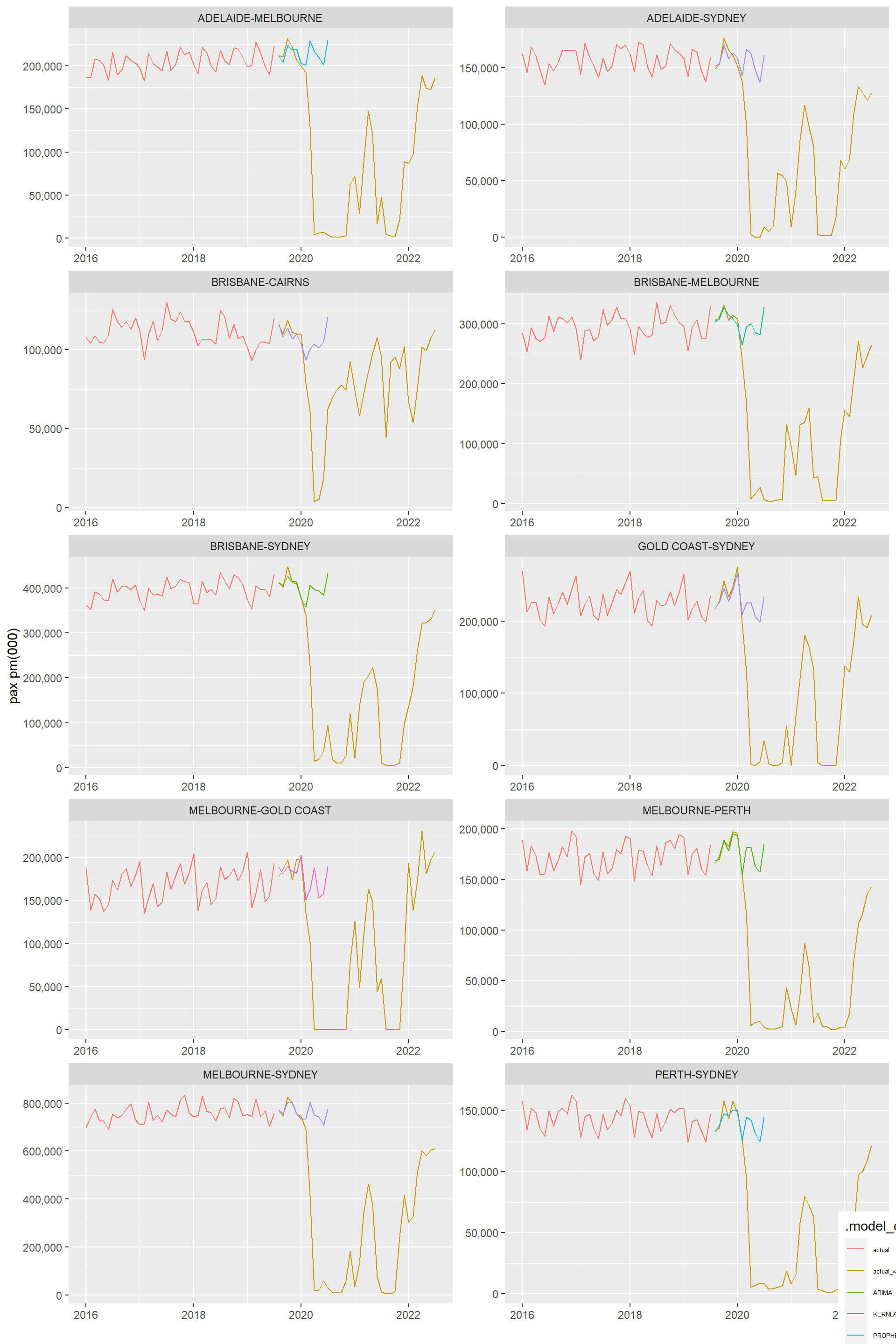

Code

  #filter((origin == city) | (dest == city) ) %>%
  # plot_modeltime_forecast(
  #   .trelliscope = FALSE,
  #   .facet_ncol  = 1
  #   
  #   #.trelliscope_params = list(width ="100%")
  #   )

Not a great performance against actuals, post covid in Feb 2020, but that is as expected! Pre-covid prediction looks good.

Accuracy of refit - Pre/post covid

Code

#unique(refit_model_by_route_acc_data$.key)

               
refit_model_by_route_acc_data <- nested_best_refit_tb_data %>% 
    # filter(.index >max(route_prep_nested_test$date),
    #        .index <= d2
    # ) %>% 
    #mutate(.key = ifelse(.key =="actual","actual","forecast")) %>%
    mutate(pax_nos = .value,
           date = .index) %>%
    bind_rows(route_prep_validation %>%
              mutate(.key = "actual",
                     passenger_trips = expm1(passenger_trips)
                     ) %>%
              select(route,date,.key, pax_nos = passenger_trips)) %>% 
    group_by(route, .key, date) %>%
    summarise(pax_nos = sum(pax_nos,na.rm = TRUE)) %>% 
    pivot_wider(names_from = .key,
              values_from  = pax_nos
  )



accuracy_predn_precovid <- refit_model_by_route_acc_data %>% 
   filter(date >  max_test,
          date <= end_precovid
   ) %>%
    summarize_accuracy_metrics(
        truth = actual_validn,
        estimate = prediction,
        metric_set = extended_forecast_accuracy_metric_set()
    ) %>% arrange(smape)

accuracy_predn_postcovid <- refit_model_by_route_acc_data %>% 
   filter(date >  end_precovid,
          date <= max_act
   ) %>%
    summarize_accuracy_metrics(
        truth = actual_validn,
        estimate = prediction,
        metric_set = extended_forecast_accuracy_metric_set()
    ) %>% arrange(smape)

For obvious reasons the accuracy of predictions against actuals is not great after the covid started (say Feb 2020), after all we did not even give the models the benefit of ‘seeing’ the covid crash. That was not the point of this analysis..although we may revisit as more post covid data is available.

We can also check accuracy at an aggregated (across all routes) level.

Code

refit_model_aggr_acc_data <- refit_model_by_route_acc_data %>% 
  group_by(date) %>% 
  summarise(actual   = sum(actual,na.rm = TRUE),
            prediction = sum(prediction,na.rm = TRUE)) 
  
accuracy_predn_agg_precovid <- refit_model_aggr_acc_data %>% 
   filter(date >  max_test,
          date <= end_precovid
   ) %>%
    summarize_accuracy_metrics(
        truth      = actual,
        estimate   = prediction,
        metric_set = extended_forecast_accuracy_metric_set()
    ) %>% arrange(smape)

  
  accuracy_predn_agg_postcovid <- refit_model_aggr_acc_data %>% 
   filter(date >  end_precovid,
          date <= max_act
   ) %>%
    summarize_accuracy_metrics(
        truth      = actual,
        estimate   = prediction,
        metric_set = extended_forecast_accuracy_metric_set()
    ) %>% arrange(smape)

agg_pred_accuracy <- accuracy_predn_agg_precovid %>% 
  mutate(period = "pre_covid") %>% 
  bind_rows(accuracy_predn_agg_postcovid %>% mutate(period = "post_covid")) %>% 
  select(period,everything())

agg_pred_accuracy %>% 
  gt::gt() %>% 
  gt::fmt_number(
    columns = !period,
    decimals = 3
  )

period	mae	mape	maape	mase	smape	rmse	rsq
pre_covid	40,507.912	1.589	1.588	0.262	1.572	63,948.883	0.989
post_covid	1,168,496.081	410.556	88.088	3.947	192.184	1,459,628.829	0.065

Obviously the pre and post covid volumes are much different so a lot of measures are not appropriate, but all look reasonable pre-covid and horrible thereafter, as expected.

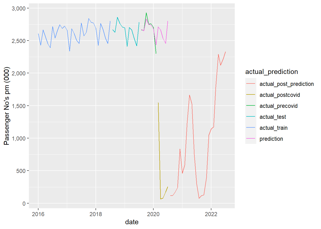
The following graph breaks the actuals into the various periods - training, testing, pre-covid prediction, post covid (Feb2020) prediction, and more recently when no prediction was attempted, so data is just for information.

So the pre-covid prediction looks good, which is really all we were asking of the models.

Now lets graph the aggregated (all routes) prediction against actuals. Actuals are colour coded to show all modelling stages. For our purposes the key is the comparison of the “prediction” to the “actual_precovid_prediction”, ie the actuals after the test period but before covid kicks in (ie pink v green line), which looks pretty good.

The rest just highlights why forecast/predictions can only go so far…

Code

refit_model_aggr_acc_data %>%
  pivot_longer(
    cols      = !date,
    names_to  = "actual_prediction",
    values_to = "pax_nos"
  ) %>%  
  mutate(actual_prediction = 
    case_when(
      actual_prediction == "prediction" ~ "prediction",
      date              <= max_train    ~ "actual_train",
      date              <= max_test     ~ "actual_test",
      date              <= end_precovid ~ "actual_precovid",
      date              <= max_pred     ~ "actual_postcovid",
      TRUE                              ~ "actual_post_prediction"
    )
  ) %>% 
  mutate(pax_nos = ifelse(pax_nos == 0, NA,pax_nos)) %>% 
  ggplot(aes(x=date, y=pax_nos/1000,colour = actual_prediction ))+
  geom_line() +
  scale_y_continuous("Passenger No's pm (000)",
    breaks = scales::breaks_extended(8),
    labels = scales::label_comma()  
  )