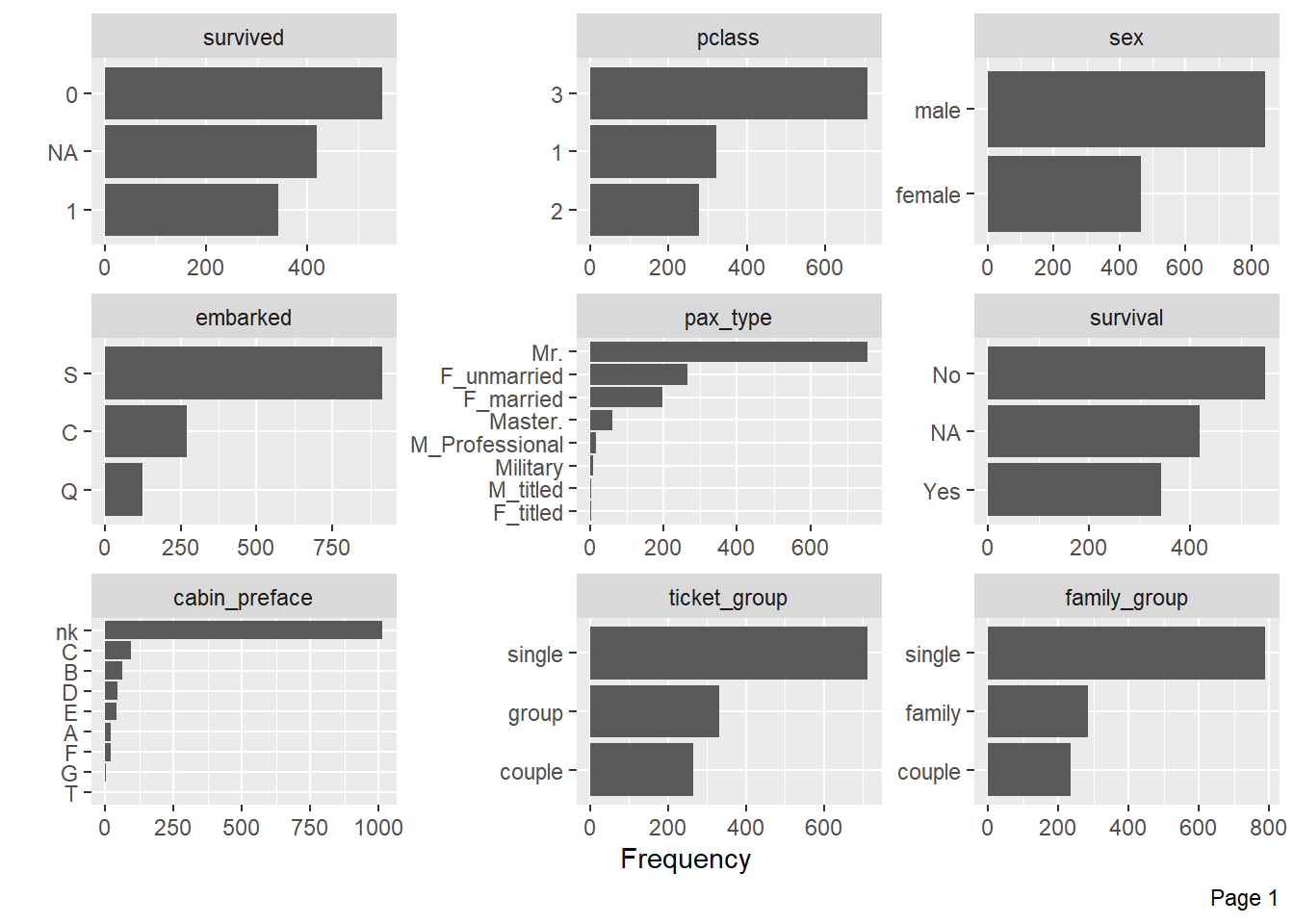
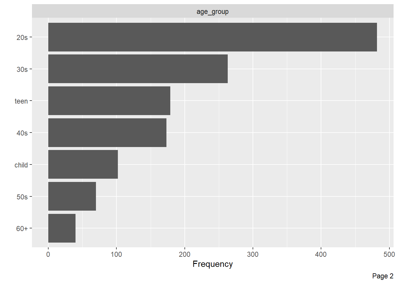
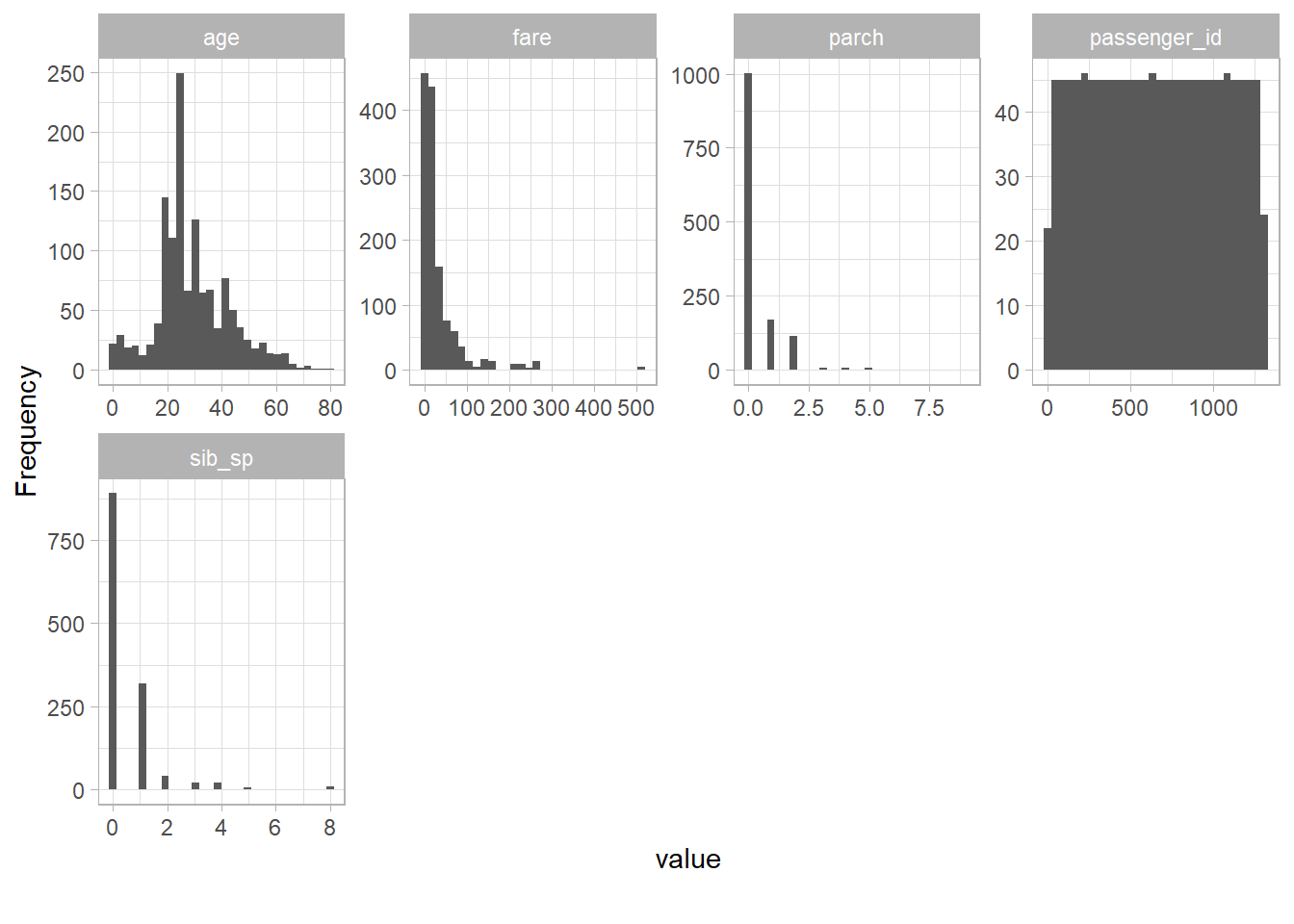
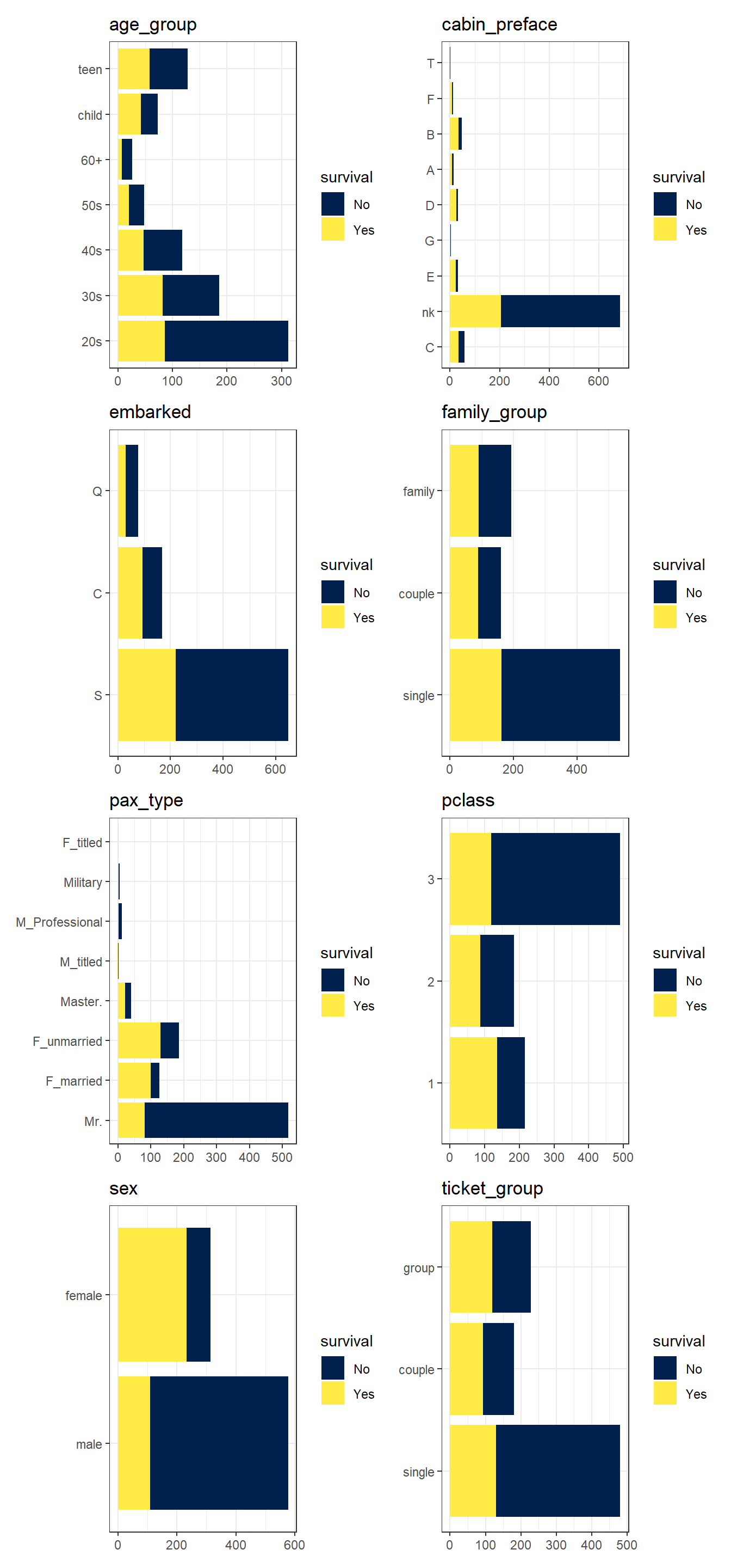
code
analysis
titanic
Author

Stephen Parton

Published

01-09-2022

0.1 Summary

This is just a first test with code in a blog using the new Quarto framework! Guess what I am using..yep Titanic, Kaggle version..

It is not very well structured as it is pretty much in the order I did it following all instructions, books and blogs from the expert TidyModels and Quarto teams at RStudio/Posit . All errors belong to me!

0.2 Final Kaggle Scores

Code
kaggle <- tibble(
  Model = c("Logistic Regression",
            "Regularised Logistic Regression",
            "Random Forest-final",
            "Random Forest-initial",
            "XG Boost",
            "Neural Net",
            "Ensemble"), 
  Score = c(.76555,.77033,.77751,.78229,.77272,.76794,.77751)
  )

kaggle %>% knitr::kable()
Model Score
Logistic Regression 0.76555
Regularised Logistic Regression 0.77033
Random Forest-final 0.77751
Random Forest-initial 0.78229
XG Boost 0.77272
Neural Net 0.76794
Ensemble 0.77751

Which when all submitted gave me a ranking of 1,872 out of 13,000 or so teams, so no grand-master!

Seems like the value mainly comes from the feature engineering and selection process (as the experts all seem to say) given the similarity in above model scores.

0.3 Review Data

0.3.1 Load Some Kaggle Data

Not the…? Yes, the Titanic again….

Code
train <- read_csv("data_raw/train.csv",show_col_types = FALSE) %>% clean_names() %>% mutate(train_test = "train")
test <- read_csv("data_raw/test.csv",show_col_types = FALSE) %>% clean_names() %>% 
  mutate(train_test = "test")
all <- train %>% bind_rows(test)

# colnames(data)
# cwd()

0.3.2 Some Initial EDA

A quick look.

Code
train %>% skim() 
Data summary
Name Piped data
Number of rows 891
Number of columns 13
_______________________
Column type frequency:
character 6
numeric 7
________________________
Group variables None

Variable type: character

skim_variable n_missing complete_rate min max empty n_unique whitespace
name 0 1.00 12 82 0 891 0
sex 0 1.00 4 6 0 2 0
ticket 0 1.00 3 18 0 681 0
cabin 687 0.23 1 15 0 147 0
embarked 2 1.00 1 1 0 3 0
train_test 0 1.00 5 5 0 1 0

Variable type: numeric

skim_variable n_missing complete_rate mean sd p0 p25 p50 p75 p100 hist
passenger_id 0 1.0 446.00 257.35 1.00 223.50 446.00 668.5 891.00 ▇▇▇▇▇
survived 0 1.0 0.38 0.49 0.00 0.00 0.00 1.0 1.00 ▇▁▁▁▅
pclass 0 1.0 2.31 0.84 1.00 2.00 3.00 3.0 3.00 ▃▁▃▁▇
age 177 0.8 29.70 14.53 0.42 20.12 28.00 38.0 80.00 ▂▇▅▂▁
sib_sp 0 1.0 0.52 1.10 0.00 0.00 0.00 1.0 8.00 ▇▁▁▁▁
parch 0 1.0 0.38 0.81 0.00 0.00 0.00 0.0 6.00 ▇▁▁▁▁
fare 0 1.0 32.20 49.69 0.00 7.91 14.45 31.0 512.33 ▇▁▁▁▁

0.3.3 Some Initial Wrangling

Code
all_proc <- all %>% 
  mutate(title = str_extract(name,"(\\w)([a-z]+)(\\.)")) %>% 
  mutate(pax_type = case_when(
    title %in% c("Miss.","Ms.","Mlle.")         ~ "F_unmarried",
    title %in% c("Mme.","Mrs.")                 ~ "F_married",
    title %in% c("Countess.","Lady.","Dona.")   ~ "F_titled",
    title %in% c("Capt.","Col.","Major.")       ~ "Military",
    title %in% c("Dr.","Rev.")                  ~ "M_Professional",
    title %in% c("Don.","Jonkheer.","Sir.")     ~ "M_titled",
    TRUE ~ title
  ),
  surname        = str_extract(name,"(\\w+)(\\,)"),
  survival       = ifelse(survived==0,"No","Yes"),
  ticket_preface = str_extract(ticket,"([:graph:]+)(\\s)"),
  ticket_preface = ifelse(is.na(ticket_preface),"none",ticket_preface),
  cabin_preface  = ifelse(is.na(cabin),"nk",
                    substr(cabin,1,1)),
  embarked       = ifelse(is.na(embarked),"S",embarked)
  ) %>% 
  group_by(pax_type,pclass) %>% 
  mutate(age     = ifelse(is.na(age),median(age,na.rm = T), age)) %>% 
  ungroup() %>% 
  add_count(ticket,name = "ticket_group") %>% 
  mutate(ticket_group = case_when(
    ticket_group == 1 ~ "single",
    ticket_group == 2 ~ "couple",
    TRUE              ~ "group"
  ),
    family_group = as.numeric(sib_sp)+as.numeric(parch)+1
  ) %>% 
  mutate(family_group = factor(
    case_when(
        family_group < 2  ~ "single",
        family_group < 3  ~ "couple",
        TRUE              ~ "family"
        ),
    ordered = TRUE)
  ) %>% 
  mutate(age_group = factor(case_when(
    age < 13      ~ "child",
    age < 20      ~ "teen",
    age < 30      ~ "20s",
    age < 40      ~ "30s",
    age < 50      ~ "40s",
    age < 60      ~ "50s",
    TRUE          ~ "60+"
    
  ),
  ordered = TRUE)
  ) %>% 
  mutate(across(where(is.character),as_factor)) %>% 
  mutate(pclass = factor(pclass,levels = c("1","2","3")),
         survived = factor(survived)
         ) %>% 
select(-c(title,ticket_preface))
  
#all_proc %>% glimpse() 

0.3.4 A bit more EDA

Code
all_proc %>% 
  select(-c(name,ticket,cabin,surname,train_test)) %>% 
  DataExplorer::plot_bar()

Code
all_proc %>% DataExplorer::plot_histogram(ggtheme = theme_light() )

0.3.5 Eyeballing Survival Graphs on Training Data

Code
no_f <- all_proc %>%
  filter(train_test == "train") %>% 
  select(passenger_id,pclass,sex,embarked,pax_type,ticket_group,family_group,age_group,cabin_preface,survival) %>% 
  droplevels() %>%
  mutate(across(where(is.factor),~ factor(.x,ordered = FALSE))) %>%
  pivot_longer(cols = c(pclass:cabin_preface)) 


g_l <- no_f %>% 
  split(.$name) %>% 
  map(~ ggplot(.,aes(y=value,fill=survival)) +
                geom_bar() +
              ggtitle(.$name) +
        theme_bw() +
        labs(x=NULL,y=NULL)+
        scale_fill_viridis_d(option = "cividis")
      
            ) 

library(patchwork)
wrap_plots(g_l, ncol = 2)

0.3.6 Split Data back to Train/Test/Validation

Code
train_proc_adj_tbl <- all_proc %>% 
  filter(train_test =="train") %>% 
  select(-c(survival))


train_split <- initial_split(train_proc_adj_tbl,strata = survived)

train_train <- training(train_split)
train_test <- testing(train_split)

0.4 Recipe-Base

Code
recipe_base <- 
  recipe(survived ~ ., data = train_train) %>% 
  update_role(passenger_id, name,surname,ticket,cabin,new_role = "ID") %>%
  step_impute_knn(all_numeric_predictors()) %>% 
  step_dummy(all_nominal_predictors()) %>%
  step_factor2string(all_nominal_predictors()) %>% 
  step_zv(all_predictors()) %>% 
  step_pca()
recipe_base
Recipe

Inputs:

      role #variables
        ID          5
   outcome          1
 predictor         13

Operations:

K-nearest neighbor imputation for all_numeric_predictors()
Dummy variables from all_nominal_predictors()
Character variables from all_nominal_predictors()
Zero variance filter on all_predictors()
PCA extraction with <none>

0.4.1 Save Files

Code
write_rds(all_proc,"artifacts/all_proc.rds")
write_rds(train_split,"artifacts/train_split.rds")
write_rds(recipe_base,"artifacts/recipe_base.rds")
# 
# all_proc <- read_rds("artifacts/all_proc.rds")
# train_split <- read_rds("artifacts/train_split.rds")
# recipe_base <- read_rds("artifacts/recipe_base.rds")

0.5 Models

0.5.1 Logistic Regression

LR Model Spec

Code
lr_spec <-  
  logistic_reg() %>% 
  set_engine("glm")

lr_spec
Logistic Regression Model Specification (classification)

Computational engine: glm 

LR Workflow

Code
lr_wflow <- 
  workflow() %>% 
  add_model(lr_spec) %>% 
  add_recipe(recipe_base)

lr_wflow
══ Workflow ════════════════════════════════════════════════════════════════════
Preprocessor: Recipe
Model: logistic_reg()

── Preprocessor ────────────────────────────────────────────────────────────────
5 Recipe Steps

• step_impute_knn()
• step_dummy()
• step_factor2string()
• step_zv()
• step_pca()

── Model ───────────────────────────────────────────────────────────────────────
Logistic Regression Model Specification (classification)

Computational engine: glm 

LR Fit Model

Code
lr_fit <- 
  lr_wflow %>% 
  last_fit(train_split)

#lr_fit

lr_final_metrics <- lr_fit %>% collect_metrics()
lr_final_metrics 
# A tibble: 2 × 4
  .metric  .estimator .estimate .config             
  <chr>    <chr>          <dbl> <chr>               
1 accuracy binary         0.799 Preprocessor1_Model1
2 roc_auc  binary         0.822 Preprocessor1_Model1
Code
#show_notes(.Last.tune.result)

LR Predict

Code
lr_test_predictions <- lr_fit %>% collect_predictions() %>% 
  rename(survived_pred = survived) %>% 
  bind_cols(train_test)
lr_test_predictions
# A tibble: 224 × 26
   id       .pred_0 .pred_1  .row .pred…¹ survi…² .config passe…³ survi…⁴ pclass
   <chr>      <dbl>   <dbl> <int> <fct>   <fct>   <chr>     <dbl> <fct>   <fct> 
 1 train/t…  0.0948 9.05e-1    10 1       1       Prepro…      10 1       2     
 2 train/t…  1.00   2.63e-7    11 0       1       Prepro…      11 1       3     
 3 train/t…  0.996  4.01e-3    14 0       0       Prepro…      14 0       3     
 4 train/t…  0.749  2.51e-1    18 0       1       Prepro…      18 1       2     
 5 train/t…  0.122  8.78e-1    20 1       1       Prepro…      20 1       3     
 6 train/t…  0.309  6.91e-1    23 1       1       Prepro…      23 1       3     
 7 train/t…  0.887  1.13e-1    28 0       0       Prepro…      28 0       1     
 8 train/t…  0.473  5.27e-1    40 1       1       Prepro…      40 1       3     
 9 train/t…  0.468  5.32e-1    41 1       0       Prepro…      41 0       3     
10 train/t…  0.862  1.38e-1    51 0       0       Prepro…      51 0       3     
# … with 214 more rows, 16 more variables: name <fct>, sex <fct>, age <dbl>,
#   sib_sp <dbl>, parch <dbl>, ticket <fct>, fare <dbl>, cabin <fct>,
#   embarked <fct>, train_test <fct>, pax_type <fct>, surname <fct>,
#   cabin_preface <fct>, ticket_group <fct>, family_group <ord>,
#   age_group <ord>, and abbreviated variable names ¹​.pred_class,
#   ²​survived_pred, ³​passenger_id, ⁴​survived

LR Performance on validation set

AUC Curve
Code
lr_test_predictions %>% 
  roc_curve(truth = survived,.pred_1,event_level="second") %>% 
  autoplot()

Confusion Matrix
Code
lr_test_predictions %>% 
  conf_mat(survived,.pred_class) %>% 
  autoplot(type = "heatmap")

LR Resampling

Code
folds <- vfold_cv(train_train, strata = survived, v=5)
#folds

control <- control_resamples(save_pred = TRUE,save_workflow = TRUE)

cores <- parallel::detectCores()
cl <- parallel::makePSOCKcluster(cores - 1)

# doParallel::registerDoParallel(cores = cores)
set.seed(1234)
lr_fit_cv <- 
  lr_wflow %>% 
  fit_resamples(folds, control = control)

#show_best(lr_fit_cv,metric= "accuracy")

#lr_fit_cv
lr_metrics_resample <- collect_metrics(lr_fit_cv)
lr_metrics_resample
# A tibble: 2 × 6
  .metric  .estimator  mean     n std_err .config             
  <chr>    <chr>      <dbl> <int>   <dbl> <chr>               
1 accuracy binary     0.823     5 0.0124  Preprocessor1_Model1
2 roc_auc  binary     0.856     5 0.00839 Preprocessor1_Model1
Code
parallel::stopCluster(cl)

Following still to be fixed!

Code
#lr_param <- extract_parameter_set_dials(lr_spec)

lr_resample_test_predictions <- collect_predictions(lr_fit_cv) %>% 
  rename(survived_pred = survived) 
#  bind_cols(testing(train_split))
lr_resample_test_predictions
# A tibble: 667 × 7
   id    .pred_0 .pred_1  .row .pred_class survived_pred .config             
   <chr>   <dbl>   <dbl> <int> <fct>       <fct>         <chr>               
 1 Fold1   0.888 0.112       2 0           0             Preprocessor1_Model1
 2 Fold1   0.756 0.244      10 0           0             Preprocessor1_Model1
 3 Fold1   0.932 0.0677     15 0           0             Preprocessor1_Model1
 4 Fold1   0.187 0.813      20 1           0             Preprocessor1_Model1
 5 Fold1   0.919 0.0810     26 0           0             Preprocessor1_Model1
 6 Fold1   0.978 0.0219     29 0           0             Preprocessor1_Model1
 7 Fold1   0.974 0.0265     34 0           0             Preprocessor1_Model1
 8 Fold1   0.993 0.00666    36 0           0             Preprocessor1_Model1
 9 Fold1   0.921 0.0793     43 0           0             Preprocessor1_Model1
10 Fold1   0.924 0.0763     44 0           0             Preprocessor1_Model1
# … with 657 more rows
Code
cl <- parallel::makePSOCKcluster(cores - 1)

set.seed(1234)
lm_fit <- lr_wflow %>% fit(data = train_proc_adj_tbl)
extract_recipe(lm_fit, estimated = TRUE)
Recipe

Inputs:

      role #variables
        ID          5
   outcome          1
 predictor         13

Training data contained 891 data points and 687 incomplete rows. 

Operations:

K-nearest neighbor imputation for age, sib_sp, parch, fare [trained]
Dummy variables from pclass, sex, embarked, train_test, pax_type, cabin_prefac... [trained]
Character variables from <none> [trained]
Zero variance filter removed train_test_test [trained]
No PCA components were extracted from <none> [trained]
Code
parallel::stopCluster(cl)

0.6 Regularised Logistic Regression - GLMNET

0.6.1 RLR Model Spec

Code
rlr_model <- 
  logistic_reg(penalty = tune(), mixture = tune()) %>% 
  set_engine("glmnet")
rlr_model
Logistic Regression Model Specification (classification)

Main Arguments:
  penalty = tune()
  mixture = tune()

Computational engine: glmnet 

0.6.2 RLR Parameter Tuning

Code
rlr_param <- extract_parameter_set_dials(rlr_model)

rlr_grid <- grid_latin_hypercube(
  penalty(),
  mixture(),
  size = 30
)
head(rlr_grid) %>% knitr::kable(digits =3)
penalty mixture
0.116 0.866
0.095 0.736
0.000 0.141
0.000 0.458
0.025 0.983
0.484 0.109

0.6.3 RLR Workflow

Code
rlr_wflow <- 
  workflow() %>% 
  add_model(rlr_model) %>% 
  add_recipe(recipe_base)
rlr_wflow
══ Workflow ════════════════════════════════════════════════════════════════════
Preprocessor: Recipe
Model: logistic_reg()

── Preprocessor ────────────────────────────────────────────────────────────────
5 Recipe Steps

• step_impute_knn()
• step_dummy()
• step_factor2string()
• step_zv()
• step_pca()

── Model ───────────────────────────────────────────────────────────────────────
Logistic Regression Model Specification (classification)

Main Arguments:
  penalty = tune()
  mixture = tune()

Computational engine: glmnet 

0.6.4 RLR Hyper-parameter Tuning

Code
# rlr_folds <- vfold_cv(training(train_split), strata = survived, v=10,repeats = 5)
# rlr_folds %>% tidy()

#doParallel::registerDoParallel(cores = cores)
cl <- parallel::makePSOCKcluster(cores - 1)

set.seed(234)
rlr_tuning_result <- tune_grid(
  rlr_wflow,
  resamples = folds,
  grid      = rlr_grid,
  control   = control_grid(save_pred = TRUE, save_workflow = TRUE)
)

rlr_tuning_metrics <- collect_metrics(rlr_tuning_result)
head(rlr_tuning_metrics) %>% knitr::kable(digits = 3)
penalty mixture .metric .estimator mean n std_err .config
0.016 0.018 accuracy binary 0.821 5 0.016 Preprocessor1_Model01
0.016 0.018 roc_auc binary 0.865 5 0.009 Preprocessor1_Model01
0.000 0.066 accuracy binary 0.825 5 0.015 Preprocessor1_Model02
0.000 0.066 roc_auc binary 0.857 5 0.008 Preprocessor1_Model02
0.000 0.070 accuracy binary 0.825 5 0.015 Preprocessor1_Model03
0.000 0.070 roc_auc binary 0.857 5 0.008 Preprocessor1_Model03
Code
parallel::stopCluster(cl)

Review hyper-parameter tuning results and select best

Code
rlr_tuning_result %>%
  collect_metrics() %>%
  filter(.metric == "accuracy") %>%
  select(mean, penalty,mixture) %>%
  pivot_longer(penalty:mixture,
               values_to = "value",
               names_to = "parameter"
  ) %>%
  ggplot(aes(value, mean, color = parameter)) +
  geom_point(alpha = 0.8, show.legend = FALSE) +
  facet_wrap(~parameter, scales = "free_x") +
  labs(x = NULL, y = "AUC")

Code
show_best(rlr_tuning_result, "accuracy")
# A tibble: 5 × 8
   penalty mixture .metric  .estimator  mean     n std_err .config              
     <dbl>   <dbl> <chr>    <chr>      <dbl> <int>   <dbl> <chr>                
1 8.86e- 3   0.923 accuracy binary     0.829     5  0.0169 Preprocessor1_Model28
2 1.36e- 9   0.141 accuracy binary     0.826     5  0.0137 Preprocessor1_Model05
3 1.30e-10   0.182 accuracy binary     0.826     5  0.0137 Preprocessor1_Model06
4 5.43e- 9   0.211 accuracy binary     0.826     5  0.0137 Preprocessor1_Model07
5 2.52e- 8   0.241 accuracy binary     0.826     5  0.0137 Preprocessor1_Model08
Code
best_rlr_auc <- select_best(rlr_tuning_result, "accuracy")
best_rlr_auc
# A tibble: 1 × 3
  penalty mixture .config              
    <dbl>   <dbl> <chr>                
1 0.00886   0.923 Preprocessor1_Model28

0.6.5 RLR Predict

Code
rlr_final_wflow <- finalize_workflow(
  rlr_wflow,
  best_rlr_auc
)

rlr_final_wflow
══ Workflow ════════════════════════════════════════════════════════════════════
Preprocessor: Recipe
Model: logistic_reg()

── Preprocessor ────────────────────────────────────────────────────────────────
5 Recipe Steps

• step_impute_knn()
• step_dummy()
• step_factor2string()
• step_zv()
• step_pca()

── Model ───────────────────────────────────────────────────────────────────────
Logistic Regression Model Specification (classification)

Main Arguments:
  penalty = 0.00885574773491923
  mixture = 0.923322001239285

Computational engine: glmnet 
Code
rlr_final_wflow %>%
  last_fit(train_split) %>%
  extract_fit_parsnip() %>%
  vip(geom = "col")

Code
rlr_final_fit <- rlr_final_wflow %>%
  last_fit(train_split)

rlr_final_metrics <- collect_metrics(rlr_final_fit)
rlr_final_metrics %>% knitr::kable()
.metric .estimator .estimate .config
accuracy binary 0.8080357 Preprocessor1_Model1
roc_auc binary 0.8424756 Preprocessor1_Model1
Code
rlr_test_predictions <- rlr_final_fit %>% collect_predictions()
rlr_test_predictions_all <- rlr_test_predictions %>% 
  bind_cols(train_test %>% select(-survived)) 


glimpse(rlr_test_predictions_all)
Rows: 224
Columns: 25
$ id            <chr> "train/test split", "train/test split", "train/test spli…
$ .pred_0       <dbl> 0.1216896, 0.8658490, 0.9641622, 0.7243443, 0.2225635, 0…
$ .pred_1       <dbl> 0.87831041, 0.13415097, 0.03583775, 0.27565575, 0.777436…
$ .row          <int> 10, 11, 14, 18, 20, 23, 28, 40, 41, 51, 54, 57, 61, 66, …
$ .pred_class   <fct> 1, 0, 0, 0, 1, 1, 0, 1, 0, 0, 1, 1, 0, 1, 0, 0, 1, 1, 0,…
$ survived      <fct> 1, 1, 0, 1, 1, 1, 0, 1, 0, 0, 1, 1, 0, 1, 0, 0, 1, 1, 1,…
$ .config       <chr> "Preprocessor1_Model1", "Preprocessor1_Model1", "Preproc…
$ passenger_id  <dbl> 10, 11, 14, 18, 20, 23, 28, 40, 41, 51, 54, 57, 61, 66, …
$ pclass        <fct> 2, 3, 3, 2, 3, 3, 1, 3, 3, 3, 2, 2, 3, 3, 2, 3, 3, 2, 3,…
$ name          <fct> "Nasser, Mrs. Nicholas (Adele Achem)", "Sandstrom, Miss.…
$ sex           <fct> female, female, male, male, female, female, male, female…
$ age           <dbl> 14, 4, 39, 30, 31, 15, 19, 14, 40, 7, 29, 21, 22, 6, 21,…
$ sib_sp        <dbl> 1, 1, 1, 0, 0, 0, 3, 1, 1, 4, 1, 0, 0, 1, 0, 0, 0, 0, 3,…
$ parch         <dbl> 0, 1, 5, 0, 0, 0, 2, 0, 0, 1, 0, 0, 0, 1, 0, 0, 0, 0, 0,…
$ ticket        <fct> 237736, PP 9549, 347082, 244373, 2649, 330923, 19950, 26…
$ fare          <dbl> 30.0708, 16.7000, 31.2750, 13.0000, 7.2250, 8.0292, 263.…
$ cabin         <fct> NA, G6, NA, NA, NA, NA, C23 C25 C27, NA, NA, NA, NA, NA,…
$ embarked      <fct> C, S, S, S, C, Q, S, C, S, S, S, S, C, C, S, S, Q, S, S,…
$ train_test    <fct> train, train, train, train, train, train, train, train, …
$ pax_type      <fct> F_married, F_unmarried, Mr., Mr., F_married, F_unmarried…
$ surname       <fct> "Nasser,", "Sandstrom,", "Andersson,", "Williams,", "Mas…
$ cabin_preface <fct> nk, G, nk, nk, nk, nk, C, nk, nk, nk, nk, nk, nk, nk, nk…
$ ticket_group  <fct> couple, group, group, single, single, single, group, cou…
$ family_group  <ord> couple, family, family, single, single, single, family, …
$ age_group     <ord> teen, child, 30s, 30s, 30s, teen, teen, teen, 40s, child…
Code
# rlr_pred <- predict(rlr_final_fit,train_2 )%>% 
#   bind_cols(predict(rlr_final_fit, train_2,type="prob")) %>% 
#   bind_cols(train_2 %>% select(survived))
# 
# rlr_pred %>% 
#   roc_auc(truth = survived, .pred_1, event_level = "second")
# 
# rlr_pred %>% 
#   roc_curve(truth = survived, .pred_1,event_level="second") %>% 
#   autoplot()
# 
# 
# rlr_metrics <- rlr_pred %>% 
# metrics(truth = survived, estimate = .pred_class) %>% 
#   filter(.metric == "accuracy")
# rlr_metrics
# survive_rlr_pred <- 
#   augment(survive_lr_fit, train_2)
# survive_rlr_pred

0.6.6 RLR Confusion Matrix

Code
rlr_test_predictions %>% conf_mat(survived,.pred_class) %>% 
  autoplot(type = "heatmap")

0.7 Random Forest

0.7.1 RF Model Spec - Ranger

Code
rf_model <- 
  rand_forest(
    trees = 1000,
    mtry  = tune(),
    min_n = tune()
    ) %>% 
  set_engine("ranger",importance = "permutation") %>% 
  set_mode("classification")

0.7.2 RF Workflow

Code
rf_wflow <- 
  workflow() %>% 
  add_model(rf_model) %>% 
  add_recipe(recipe_base)

0.7.3 RF Tuning - Initial

Code
cl <- parallel::makePSOCKcluster(cores - 1)

set.seed(1234)
rf_tuning_result <- tune_grid(
  rf_wflow,
  resamples = folds,
  grid = 20
)
parallel::stopCluster(cl)

rf_tuning_result
# Tuning results
# 5-fold cross-validation using stratification 
# A tibble: 5 × 4
  splits            id    .metrics          .notes          
  <list>            <chr> <list>            <list>          
1 <split [532/135]> Fold1 <tibble [40 × 6]> <tibble [0 × 3]>
2 <split [534/133]> Fold2 <tibble [40 × 6]> <tibble [0 × 3]>
3 <split [534/133]> Fold3 <tibble [40 × 6]> <tibble [0 × 3]>
4 <split [534/133]> Fold4 <tibble [40 × 6]> <tibble [0 × 3]>
5 <split [534/133]> Fold5 <tibble [40 × 6]> <tibble [0 × 3]>
Code
rf_tuning_result %>% 
  collect_metrics() %>% 
  filter(.metric == "accuracy") %>% 
  select(mean,min_n,mtry) %>% 
  pivot_longer(min_n:mtry) %>% 
  ggplot(aes(value, mean, color = name)) +
  geom_point(show.legend = FALSE) +
  facet_wrap(~name, scales = "free_x") +
  labs(x = NULL, y = "Accuracy")

Bit hard to make much of it, but say min_n between 10 and 40 and mtry between 10 and 30?

Code
rf_grid <- grid_regular(
  mtry(range = c(5, 40)),
  min_n(range = c(5, 30)),
  levels = 5
)

rf_grid
# A tibble: 25 × 2
    mtry min_n
   <int> <int>
 1     5     5
 2    13     5
 3    22     5
 4    31     5
 5    40     5
 6     5    11
 7    13    11
 8    22    11
 9    31    11
10    40    11
# … with 15 more rows

0.7.4 RF Graph Results

Code
cl <- parallel::makePSOCKcluster(cores - 1)


set.seed(1234)
rf_grid_tune <- tune_grid(
  rf_wflow,
  resamples = folds,
  grid = rf_grid
)
rf_grid_tune
# Tuning results
# 5-fold cross-validation using stratification 
# A tibble: 5 × 4
  splits            id    .metrics          .notes          
  <list>            <chr> <list>            <list>          
1 <split [532/135]> Fold1 <tibble [50 × 6]> <tibble [5 × 3]>
2 <split [534/133]> Fold2 <tibble [50 × 6]> <tibble [5 × 3]>
3 <split [534/133]> Fold3 <tibble [50 × 6]> <tibble [5 × 3]>
4 <split [534/133]> Fold4 <tibble [50 × 6]> <tibble [5 × 3]>
5 <split [534/133]> Fold5 <tibble [50 × 6]> <tibble [5 × 3]>

There were issues with some computations:

  - Warning(s) x10: 40 columns were requested but there were 33 predictors in the dat...   - Warning(s) x15: 40 columns were requested but there were 33 predictors in the dat...

Run `show_notes(.Last.tune.result)` for more information.
Code
parallel::stopCluster(cl)

rf_grid_tune %>%
  collect_metrics() %>%
  filter(.metric == "accuracy") %>%
  mutate(min_n = factor(min_n)) %>%
  ggplot(aes(mtry, mean, color = min_n)) +
  geom_line(alpha = 0.5, size = 1.5) +
  geom_point() +
  labs(y = "Accuracy")

Well that’s interesting, lets see what tune thinks is best

Code
rf_best_params <- select_best(rf_grid_tune,"accuracy")
rf_best_params %>% knitr::kable()
mtry min_n .config
31 17 Preprocessor1_Model14

0.7.5 RF Final Model

Code
rf_final_model <- finalize_model(
  rf_model,
  rf_best_params
)
rf_final_model
Random Forest Model Specification (classification)

Main Arguments:
  mtry = 31
  trees = 1000
  min_n = 17

Engine-Specific Arguments:
  importance = permutation

Computational engine: ranger 

0.7.6 RF Final Workflow

Code
rf_final_wflow <- finalize_workflow(
  rf_wflow,
  rf_best_params
)

rf_final_wflow
══ Workflow ════════════════════════════════════════════════════════════════════
Preprocessor: Recipe
Model: rand_forest()

── Preprocessor ────────────────────────────────────────────────────────────────
5 Recipe Steps

• step_impute_knn()
• step_dummy()
• step_factor2string()
• step_zv()
• step_pca()

── Model ───────────────────────────────────────────────────────────────────────
Random Forest Model Specification (classification)

Main Arguments:
  mtry = 31
  trees = 1000
  min_n = 17

Engine-Specific Arguments:
  importance = permutation

Computational engine: ranger 

0.7.7 RF Parameter Importance

Code
rf_final_wflow %>%
  fit(data = train_proc_adj_tbl) %>%
  extract_fit_parsnip() %>%
  vip(geom = "point")

0.7.8 RF Final Fit

Code
rf_final_fit <- 
  rf_final_wflow %>% 
  last_fit(train_split)

rf_final_metrics <- collect_metrics(rf_final_fit)
rf_final_metrics
# A tibble: 2 × 4
  .metric  .estimator .estimate .config             
  <chr>    <chr>          <dbl> <chr>               
1 accuracy binary         0.821 Preprocessor1_Model1
2 roc_auc  binary         0.874 Preprocessor1_Model1

0.7.9 RF Predict

Code
# rf_final_fit <- rf_wflow %>% fit(train_test)
# class(rf_final_fit)

 rf_test_predictions <- 
   collect_predictions(rf_final_fit)
   # fit(rf_final_wflow,train_train) %>% 
   # predict(rf_final_wflow, new_data = train_test) %>% 
   #bind_cols(predict(rf_final_wflow, train_test,type = "prob")) %>% 
   #bind_cols(train_test %>% select(survived))

 
 head(rf_test_predictions)
# A tibble: 6 × 7
  id               .pred_0 .pred_1  .row .pred_class survived .config           
  <chr>              <dbl>   <dbl> <int> <fct>       <fct>    <chr>             
1 train/test split  0.0101   0.990    10 1           1        Preprocessor1_Mod…
2 train/test split  0.386    0.614    11 1           1        Preprocessor1_Mod…
3 train/test split  0.703    0.297    14 0           0        Preprocessor1_Mod…
4 train/test split  0.884    0.116    18 0           1        Preprocessor1_Mod…
5 train/test split  0.370    0.630    20 1           1        Preprocessor1_Mod…
6 train/test split  0.598    0.402    23 0           1        Preprocessor1_Mod…

0.7.10 RF Performance on Test Set

Code
# rf_test_predictions %>% 
#   roc_auc(truth = survived, .pred_1,event_level = "second")

rf_metrics_accuracy <- rf_test_predictions %>% 
  metrics(truth = survived, estimate = .pred_class) %>% 
  filter(.metric == "accuracy")
rf_metrics_accuracy
# A tibble: 1 × 3
  .metric  .estimator .estimate
  <chr>    <chr>          <dbl>
1 accuracy binary         0.821
Code
rf_test_predictions %>% 
  roc_curve(truth = survived, .pred_1,event_level = "second") %>% 
  autoplot()

0.7.11 RF Confusion Matrix

Code
rf_test_predictions %>% conf_mat(survived,.pred_class) %>% 
  autoplot(type = "heatmap")

0.8 XG Boost - Usemodel

0.8.1 XGB - Usemodel Library specs

Code
library(usemodels)

use_xgboost(survived ~ .,
            data=train_train,
            verbose = TRUE
  
)
xgboost_recipe <- 
  recipe(formula = survived ~ ., data = train_train) %>% 
  step_novel(all_nominal_predictors()) %>% 
  ## This model requires the predictors to be numeric. The most common 
  ## method to convert qualitative predictors to numeric is to create 
  ## binary indicator variables (aka dummy variables) from these 
  ## predictors. However, for this model, binary indicator variables can be 
  ## made for each of the levels of the factors (known as 'one-hot 
  ## encoding'). 
  step_dummy(all_nominal_predictors(), one_hot = TRUE) %>% 
  step_zv(all_predictors()) 

xgboost_spec <- 
  boost_tree(trees = tune(), min_n = tune(), tree_depth = tune(), learn_rate = tune(), 
    loss_reduction = tune(), sample_size = tune()) %>% 
  set_mode("classification") %>% 
  set_engine("xgboost") 

xgboost_workflow <- 
  workflow() %>% 
  add_recipe(xgboost_recipe) %>% 
  add_model(xgboost_spec) 

set.seed(19336)
xgboost_tune <-
  tune_grid(xgboost_workflow, resamples = stop("add your rsample object"), grid = stop("add number of candidate points"))

0.8.2 XGB - Parameters

This grid is used for both versions of XG Boost.

Code
xgb_grid <- grid_latin_hypercube(
  tree_depth(),
  min_n(),
  trees(),
  loss_reduction(),
  sample_size = sample_prop(),
  finalize(mtry(), train_train),
  learn_rate(),
  size = 30
)

head(xgb_grid)
# A tibble: 6 × 7
  tree_depth min_n trees loss_reduction sample_size  mtry    learn_rate
       <int> <int> <int>          <dbl>       <dbl> <int>         <dbl>
1         14    30  1603   0.0230             0.806    13 0.00985      
2         11     9    22   0.0000361          0.983     3 0.0000469    
3          1    17   848   0.00581            0.539    11 0.00559      
4         10     8  1097   0.00000104         0.652     8 0.00000000128
5         11    19  1422   1.00               0.283     6 0.00124      
6         15    32  1007   0.0000000318       0.919    15 0.00000608   
Code
xgboost_usemodel_recipe <- 
  recipe(formula = survived ~ ., data = train_train) %>% 
  step_novel(all_nominal_predictors()) %>% 
  ## This model requires the predictors to be numeric. The most common 
  ## method to convert qualitative predictors to numeric is to create 
  ## binary indicator variables (aka dummy variables) from these 
  ## predictors. However, for this model, binary indicator variables can be 
  ## made for each of the levels of the factors (known as 'one-hot 
  ## encoding'). 
  step_dummy(all_nominal_predictors(), one_hot = TRUE) %>% 
  step_zv(all_predictors()) 

xgboost_usemodel_model <- 
  boost_tree(trees = tune(), mtry = tune(),min_n = tune(), tree_depth = tune(), learn_rate = tune(), 
    loss_reduction = tune(), sample_size = tune()) %>% 
  set_mode("classification") %>% 
  set_engine("xgboost") 

xgboost_usemodel_wflow <- 
  workflow() %>% 
  add_recipe(xgboost_usemodel_recipe) %>% 
  add_model(xgboost_usemodel_model) 

#doParallel::registerDoParallel(cores = cores)
cl <- parallel::makePSOCKcluster(cores - 1)

set.seed(1234)
xgboost_usemodel_tune <-
  tune_grid(xgboost_usemodel_wflow, resamples = folds, grid = xgb_grid)

parallel::stopCluster(cl)

0.8.3 XGB - Usemodel Best Parameter Settings

Code
xgb_tuning_metrics_usemodel <- collect_metrics(xgboost_usemodel_tune)
xgb_tuning_metrics_usemodel
# A tibble: 60 × 13
    mtry trees min_n tree_depth learn_r…¹ loss_r…² sampl…³ .metric .esti…⁴  mean
   <int> <int> <int>      <int>     <dbl>    <dbl>   <dbl> <chr>   <chr>   <dbl>
 1    11   848    17          1   5.59e-3 5.81e- 3   0.539 accura… binary  0.708
 2    11   848    17          1   5.59e-3 5.81e- 3   0.539 roc_auc binary  0.823
 3     9  1145    10          2   5.20e-8 1.60e- 1   0.866 accura… binary  0.702
 4     9  1145    10          2   5.20e-8 1.60e- 1   0.866 roc_auc binary  0.821
 5    17   740    15          2   8.39e-2 6.64e- 9   0.252 accura… binary  0.743
 6    17   740    15          2   8.39e-2 6.64e- 9   0.252 roc_auc binary  0.776
 7    12   690    38          2   3.89e-9 5.16e-10   0.146 accura… binary  0.616
 8    12   690    38          2   3.89e-9 5.16e-10   0.146 roc_auc binary  0.5  
 9    10  1314    11          3   1.72e-5 1.25e- 1   0.163 accura… binary  0.616
10    10  1314    11          3   1.72e-5 1.25e- 1   0.163 roc_auc binary  0.757
# … with 50 more rows, 3 more variables: n <int>, std_err <dbl>, .config <chr>,
#   and abbreviated variable names ¹​learn_rate, ²​loss_reduction, ³​sample_size,
#   ⁴​.estimator
Code
xgboost_usemodel_tune %>%
  collect_metrics() %>%
  filter(.metric == "accuracy") %>%
  select(mean, mtry:sample_size) %>%
  pivot_longer(mtry:sample_size,
               values_to = "value",
               names_to = "parameter"
  ) %>%
  ggplot(aes(value, mean, color = parameter)) +
  geom_point(alpha = 0.8, show.legend = FALSE) +
  facet_wrap(~parameter, scales = "free_x") +
  labs(x = NULL, y = "Accuracy")

Now select best from above

Code
show_best(xgboost_usemodel_tune, "accuracy")
# A tibble: 5 × 13
   mtry trees min_n tree_d…¹ learn…² loss_…³ sampl…⁴ .metric .esti…⁵  mean     n
  <int> <int> <int>    <int>   <dbl>   <dbl>   <dbl> <chr>   <chr>   <dbl> <int>
1    13  1603    30       14 9.85e-3 2.30e-2   0.806 accura… binary  0.766     5
2     4  1982     4       15 4.01e-2 5.53e-8   0.393 accura… binary  0.754     5
3    17   740    15        2 8.39e-2 6.64e-9   0.252 accura… binary  0.743     5
4    11   848    17        1 5.59e-3 5.81e-3   0.539 accura… binary  0.708     5
5     9  1145    10        2 5.20e-8 1.60e-1   0.866 accura… binary  0.702     5
# … with 2 more variables: std_err <dbl>, .config <chr>, and abbreviated
#   variable names ¹​tree_depth, ²​learn_rate, ³​loss_reduction, ⁴​sample_size,
#   ⁵​.estimator
Code
xgb_usemodel_best_params <- select_best(xgboost_usemodel_tune, "accuracy")
xgb_usemodel_best_params
# A tibble: 1 × 8
   mtry trees min_n tree_depth learn_rate loss_reduction sample_size .config    
  <int> <int> <int>      <int>      <dbl>          <dbl>       <dbl> <chr>      
1    13  1603    30         14    0.00985         0.0230       0.806 Preprocess…
Code
xgb_usemodel_final_wflow <- finalize_workflow(
  xgboost_usemodel_wflow,
  xgb_usemodel_best_params
)

xgb_usemodel_final_wflow
══ Workflow ════════════════════════════════════════════════════════════════════
Preprocessor: Recipe
Model: boost_tree()

── Preprocessor ────────────────────────────────────────────────────────────────
3 Recipe Steps

• step_novel()
• step_dummy()
• step_zv()

── Model ───────────────────────────────────────────────────────────────────────
Boosted Tree Model Specification (classification)

Main Arguments:
  mtry = 13
  trees = 1603
  min_n = 30
  tree_depth = 14
  learn_rate = 0.00985014124434902
  loss_reduction = 0.0230337047700143
  sample_size = 0.80635308077326

Computational engine: xgboost 

0.8.4 XGB - Usemodel Parameter Ranking - VIP

Code
xgb_usemodel_final_wflow %>%
  fit(data = train_train) %>%
  extract_fit_parsnip() %>%
  vip(geom = "point")

0.8.5 XGB - Usemodel Performance

XGB - Usemodel Accuracy Measured on Test Set

Code
cl <- parallel::makePSOCKcluster(cores - 1)

set.seed(1234)
xgb_usemodel_final_res <- last_fit(xgb_usemodel_final_wflow, train_split)
xgb_usemodel_final_res
# Resampling results
# Manual resampling 
# A tibble: 1 × 6
  splits            id               .metrics .notes   .predictions .workflow 
  <list>            <chr>            <list>   <list>   <list>       <list>    
1 <split [667/224]> train/test split <tibble> <tibble> <tibble>     <workflow>

There were issues with some computations:

  - Warning(s) x2: There are new levels in a factor: NA

Run `show_notes(.Last.tune.result)` for more information.
Code
xgb_usemodel_final_metrics <- collect_metrics(xgb_usemodel_final_res)
xgb_usemodel_final_metrics
# A tibble: 2 × 4
  .metric  .estimator .estimate .config             
  <chr>    <chr>          <dbl> <chr>               
1 accuracy binary         0.670 Preprocessor1_Model1
2 roc_auc  binary         0.797 Preprocessor1_Model1
Code
parallel::stopCluster(cl)

XGB - Usemodel AUC on Test Set (within train)

Code
xgb_usemodel_final_res %>%
  collect_predictions() %>%
  roc_curve( truth = survived,.pred_1, event_level = "second") %>%
  ggplot(aes(x = 1-specificity, y = sensitivity)) +
  geom_line(size = 1.5, color = "midnightblue") +
  geom_abline(
    lty = 2, alpha = 0.5,
    color = "gray50",
    size = 1.2
  )

Code
xgb_usemodel_test_predictions <- collect_predictions(xgb_usemodel_final_res)
head(xgb_usemodel_test_predictions)
# A tibble: 6 × 7
  id               .pred_0 .pred_1  .row .pred_class survived .config           
  <chr>              <dbl>   <dbl> <int> <fct>       <fct>    <chr>             
1 train/test split   0.534   0.466    10 0           1        Preprocessor1_Mod…
2 train/test split   0.291   0.709    11 1           1        Preprocessor1_Mod…
3 train/test split   0.733   0.267    14 0           0        Preprocessor1_Mod…
4 train/test split   0.736   0.264    18 0           1        Preprocessor1_Mod…
5 train/test split   0.640   0.360    20 0           1        Preprocessor1_Mod…
6 train/test split   0.625   0.375    23 0           1        Preprocessor1_Mod…

0.8.6 XGB - Usemodel Confusion Matrix

Code
xgb_usemodel_test_predictions %>% conf_mat(survived,.pred_class) %>% 
  autoplot(type = "heatmap")

0.9 XG Boost - Base Recipe

0.9.1 XGB Model Spec

Code
xgb_model <- 
  boost_tree(
    trees = tune(),
    tree_depth = tune(),
    min_n = tune(),
    loss_reduction = tune(),
    sample_size = tune(),
    mtry = tune(),
    learn_rate = tune()) %>% 
  set_engine("xgboost") %>% 
  set_mode("classification")

xgb_model
Boosted Tree Model Specification (classification)

Main Arguments:
  mtry = tune()
  trees = tune()
  min_n = tune()
  tree_depth = tune()
  learn_rate = tune()
  loss_reduction = tune()
  sample_size = tune()

Computational engine: xgboost 

0.9.2 XGB Workflow

Code
xgb_wflow <- 
  workflow() %>% 
  add_model(xgb_model) %>% 
  add_recipe(recipe_base)

0.9.3 XGB Hyper-Parameter Tuning

Code
# xgb_folds <- vfold_cv(training(train_split), strata = survived)
# xgb_folds


#doParallel::registerDoParallel(cores = cores)

set.seed(1234)
cl <- parallel::makePSOCKcluster(cores - 1)

xgb_tuning_result <- tune_grid(
  xgb_wflow,
  resamples = folds,
  grid      = xgb_grid,
  control  = control_grid(save_pred = TRUE,save_workflow = TRUE)
)
xgb_tuning_result
# Tuning results
# 5-fold cross-validation using stratification 
# A tibble: 5 × 5
  splits            id    .metrics           .notes           .predictions
  <list>            <chr> <list>             <list>           <list>      
1 <split [532/135]> Fold1 <tibble [60 × 11]> <tibble [0 × 3]> <tibble>    
2 <split [534/133]> Fold2 <tibble [60 × 11]> <tibble [0 × 3]> <tibble>    
3 <split [534/133]> Fold3 <tibble [60 × 11]> <tibble [0 × 3]> <tibble>    
4 <split [534/133]> Fold4 <tibble [60 × 11]> <tibble [0 × 3]> <tibble>    
5 <split [534/133]> Fold5 <tibble [60 × 11]> <tibble [0 × 3]> <tibble>    
Code
parallel::stopCluster(cl)
Code
xgb_tuning_metrics <- collect_metrics(xgb_tuning_result)
xgb_tuning_metrics
# A tibble: 60 × 13
    mtry trees min_n tree_depth learn_r…¹ loss_r…² sampl…³ .metric .esti…⁴  mean
   <int> <int> <int>      <int>     <dbl>    <dbl>   <dbl> <chr>   <chr>   <dbl>
 1    11   848    17          1   5.59e-3 5.81e- 3   0.539 accura… binary  0.775
 2    11   848    17          1   5.59e-3 5.81e- 3   0.539 roc_auc binary  0.844
 3     9  1145    10          2   5.20e-8 1.60e- 1   0.866 accura… binary  0.775
 4     9  1145    10          2   5.20e-8 1.60e- 1   0.866 roc_auc binary  0.842
 5    17   740    15          2   8.39e-2 6.64e- 9   0.252 accura… binary  0.718
 6    17   740    15          2   8.39e-2 6.64e- 9   0.252 roc_auc binary  0.753
 7    12   690    38          2   3.89e-9 5.16e-10   0.146 accura… binary  0.616
 8    12   690    38          2   3.89e-9 5.16e-10   0.146 roc_auc binary  0.5  
 9    10  1314    11          3   1.72e-5 1.25e- 1   0.163 accura… binary  0.616
10    10  1314    11          3   1.72e-5 1.25e- 1   0.163 roc_auc binary  0.721
# … with 50 more rows, 3 more variables: n <int>, std_err <dbl>, .config <chr>,
#   and abbreviated variable names ¹​learn_rate, ²​loss_reduction, ³​sample_size,
#   ⁴​.estimator
Code
xgb_tuning_result %>%
  collect_metrics() %>%
  filter(.metric == "accuracy") %>%
  select(mean, mtry:sample_size) %>%
  pivot_longer(mtry:sample_size,
               values_to = "value",
               names_to = "parameter"
  ) %>%
  ggplot(aes(value, mean, color = parameter)) +
  geom_point(alpha = 0.8, show.legend = FALSE) +
  facet_wrap(~parameter, scales = "free_x") +
  labs(x = NULL, y = "AUC")

XGB Best Parameters then Finalise Workflow

Code
show_best(xgb_tuning_result, "accuracy")
# A tibble: 5 × 13
   mtry trees min_n tree_d…¹ learn…² loss_…³ sampl…⁴ .metric .esti…⁵  mean     n
  <int> <int> <int>    <int>   <dbl>   <dbl>   <dbl> <chr>   <chr>   <dbl> <int>
1     4  1982     4       15 4.01e-2 5.53e-8   0.393 accura… binary  0.814     5
2    15  1689     7       13 2.02e-9 5.67e-6   0.958 accura… binary  0.784     5
3    16  1549     6        7 1.36e-4 4.92e-4   0.463 accura… binary  0.783     5
4    19   259    16        9 6.05e-7 1.64e-4   0.735 accura… binary  0.781     5
5    13  1603    30       14 9.85e-3 2.30e-2   0.806 accura… binary  0.780     5
# … with 2 more variables: std_err <dbl>, .config <chr>, and abbreviated
#   variable names ¹​tree_depth, ²​learn_rate, ³​loss_reduction, ⁴​sample_size,
#   ⁵​.estimator
Code
xgb_best_params <- select_best(xgb_tuning_result, "accuracy")
xgb_best_params
# A tibble: 1 × 8
   mtry trees min_n tree_depth learn_rate loss_reduction sample_size .config    
  <int> <int> <int>      <int>      <dbl>          <dbl>       <dbl> <chr>      
1     4  1982     4         15     0.0401   0.0000000553       0.393 Preprocess…
Code
xgb_final_wflow <- finalize_workflow(
  xgb_wflow,
  xgb_best_params
)

xgb_final_wflow
══ Workflow ════════════════════════════════════════════════════════════════════
Preprocessor: Recipe
Model: boost_tree()

── Preprocessor ────────────────────────────────────────────────────────────────
5 Recipe Steps

• step_impute_knn()
• step_dummy()
• step_factor2string()
• step_zv()
• step_pca()

── Model ───────────────────────────────────────────────────────────────────────
Boosted Tree Model Specification (classification)

Main Arguments:
  mtry = 4
  trees = 1982
  min_n = 4
  tree_depth = 15
  learn_rate = 0.0400670375292599
  loss_reduction = 5.52655767061452e-08
  sample_size = 0.392634701682255

Computational engine: xgboost 
Code
xgb_final_wflow %>%
  fit(data = train_train) %>%
  extract_fit_parsnip() %>%
  vip(geom = "point")

0.9.4 XGB Performance on Training Test Set

XGB Accuracy Measured on Test Set

Code
xgb_final_res <- last_fit(xgb_final_wflow, train_split)
xgb_final_res
# Resampling results
# Manual resampling 
# A tibble: 1 × 6
  splits            id               .metrics .notes   .predictions .workflow 
  <list>            <chr>            <list>   <list>   <list>       <list>    
1 <split [667/224]> train/test split <tibble> <tibble> <tibble>     <workflow>
Code
xgb_final_metrics <- collect_metrics(xgb_final_res)
xgb_final_metrics
# A tibble: 2 × 4
  .metric  .estimator .estimate .config             
  <chr>    <chr>          <dbl> <chr>               
1 accuracy binary         0.839 Preprocessor1_Model1
2 roc_auc  binary         0.870 Preprocessor1_Model1

XGB AUC on Test Set (within train)

Code
xgb_final_res %>%
  collect_predictions() %>%
  roc_curve( truth = survived,.pred_1, event_level = "second") %>%
  ggplot(aes(x = 1-specificity, y = sensitivity)) +
  geom_line(size = 1.5, color = "midnightblue") +
  geom_abline(
    lty = 2, alpha = 0.5,
    color = "gray50",
    size = 1.2
  )

Code
xgb_test_predictions <- collect_predictions(xgb_final_res)
head(xgb_test_predictions)
# A tibble: 6 × 7
  id               .pred_0 .pred_1  .row .pred_class survived .config           
  <chr>              <dbl>   <dbl> <int> <fct>       <fct>    <chr>             
1 train/test split  0.0609  0.939     10 1           1        Preprocessor1_Mod…
2 train/test split  0.346   0.654     11 1           1        Preprocessor1_Mod…
3 train/test split  0.968   0.0321    14 0           0        Preprocessor1_Mod…
4 train/test split  0.845   0.155     18 0           1        Preprocessor1_Mod…
5 train/test split  0.385   0.615     20 1           1        Preprocessor1_Mod…
6 train/test split  0.319   0.681     23 1           1        Preprocessor1_Mod…

0.9.5 XGB Confusion Matrix

Code
xgb_test_predictions %>% conf_mat(survived,.pred_class) %>% 
  autoplot(type = "heatmap")

0.10 Neural Net

0.10.1 NN Model

Code
nnet_model <- 
   mlp(hidden_units = tune(), penalty = tune(), epochs = tune()) %>% 
   set_engine("nnet", MaxNWts = 2600) %>% 
   set_mode("classification")

nnet_model %>% translate()
Single Layer Neural Network Model Specification (classification)

Main Arguments:
  hidden_units = tune()
  penalty = tune()
  epochs = tune()

Engine-Specific Arguments:
  MaxNWts = 2600

Computational engine: nnet 

Model fit template:
nnet::nnet(formula = missing_arg(), data = missing_arg(), size = tune(), 
    decay = tune(), maxit = tune(), MaxNWts = 2600, trace = FALSE, 
    linout = FALSE)

0.10.2 NN Workflow

Code
nnet_wflow <- workflow() %>% 
  add_model(nnet_model) %>% 
  add_recipe(recipe_base)

0.10.3 NN Parameters

Code
nnet_grid <- grid_latin_hypercube(
  hidden_units(),
  penalty (),
  epochs ()
)

head(nnet_grid) 
# A tibble: 3 × 3
  hidden_units  penalty epochs
         <int>    <dbl>  <int>
1            7 7.66e- 5    944
2            6 6.36e-10    524
3            2 1.80e- 3    146

0.10.4 NN Hyper-Parameter Tuning

Code
# nnet_folds <- vfold_cv(train_train, strata = survived)
# nnet_folds


# doParallel::registerDoParallel(cores = cores)
cl <- parallel::makePSOCKcluster(cores - 1)

set.seed(1234)
nnet_tuning_result <- tune_grid(
  nnet_wflow,
  resamples = folds,
  grid      = nnet_grid,
  control   = control_grid(save_pred = TRUE,save_workflow = TRUE)
)
nnet_tuning_result
# Tuning results
# 5-fold cross-validation using stratification 
# A tibble: 5 × 5
  splits            id    .metrics         .notes           .predictions      
  <list>            <chr> <list>           <list>           <list>            
1 <split [532/135]> Fold1 <tibble [6 × 7]> <tibble [0 × 3]> <tibble [405 × 9]>
2 <split [534/133]> Fold2 <tibble [6 × 7]> <tibble [0 × 3]> <tibble [399 × 9]>
3 <split [534/133]> Fold3 <tibble [6 × 7]> <tibble [0 × 3]> <tibble [399 × 9]>
4 <split [534/133]> Fold4 <tibble [6 × 7]> <tibble [0 × 3]> <tibble [399 × 9]>
5 <split [534/133]> Fold5 <tibble [6 × 7]> <tibble [0 × 3]> <tibble [399 × 9]>
Code
parallel::stopCluster(cl)

0.10.5 NN Best Parameters and Finalise Workflow

Code
show_best(nnet_tuning_result, "accuracy")
# A tibble: 3 × 9
  hidden_units  penalty epochs .metric  .estimator  mean     n std_err .config  
         <int>    <dbl>  <int> <chr>    <chr>      <dbl> <int>   <dbl> <chr>    
1            2 1.80e- 3    146 accuracy binary     0.820     5  0.0161 Preproce…
2            7 7.66e- 5    944 accuracy binary     0.776     5  0.0372 Preproce…
3            6 6.36e-10    524 accuracy binary     0.766     5  0.0334 Preproce…
Code
nn_best_params <- select_best(nnet_tuning_result, "accuracy")

nnet_best_auc <- select_best(xgb_tuning_result, "accuracy")
nnet_best_auc
# A tibble: 1 × 8
   mtry trees min_n tree_depth learn_rate loss_reduction sample_size .config    
  <int> <int> <int>      <int>      <dbl>          <dbl>       <dbl> <chr>      
1     4  1982     4         15     0.0401   0.0000000553       0.393 Preprocess…
Code
nnet_final_wflow <- finalize_workflow(
  nnet_wflow,
  nn_best_params
)

nnet_final_wflow
══ Workflow ════════════════════════════════════════════════════════════════════
Preprocessor: Recipe
Model: mlp()

── Preprocessor ────────────────────────────────────────────────────────────────
5 Recipe Steps

• step_impute_knn()
• step_dummy()
• step_factor2string()
• step_zv()
• step_pca()

── Model ───────────────────────────────────────────────────────────────────────
Single Layer Neural Network Model Specification (classification)

Main Arguments:
  hidden_units = 2
  penalty = 0.00180188446786651
  epochs = 146

Engine-Specific Arguments:
  MaxNWts = 2600

Computational engine: nnet 
Code
nnet_final_wflow %>%
  fit(data = train_train) %>%
  extract_fit_parsnip() %>%
  vip(geom = "point")

0.10.6 NN Accuracy - Train/Test Set

Code
nnet_tuning_metrics <- collect_metrics(nnet_tuning_result)
nnet_tuning_metrics
# A tibble: 6 × 9
  hidden_units  penalty epochs .metric  .estimator  mean     n std_err .config  
         <int>    <dbl>  <int> <chr>    <chr>      <dbl> <int>   <dbl> <chr>    
1            7 7.66e- 5    944 accuracy binary     0.776     5  0.0372 Preproce…
2            7 7.66e- 5    944 roc_auc  binary     0.788     5  0.0395 Preproce…
3            6 6.36e-10    524 accuracy binary     0.766     5  0.0334 Preproce…
4            6 6.36e-10    524 roc_auc  binary     0.779     5  0.0421 Preproce…
5            2 1.80e- 3    146 accuracy binary     0.820     5  0.0161 Preproce…
6            2 1.80e- 3    146 roc_auc  binary     0.865     5  0.0153 Preproce…
Code
nnet_final_res <- last_fit(nnet_final_wflow, train_split)
nnet_final_res
# Resampling results
# Manual resampling 
# A tibble: 1 × 6
  splits            id               .metrics .notes   .predictions .workflow 
  <list>            <chr>            <list>   <list>   <list>       <list>    
1 <split [667/224]> train/test split <tibble> <tibble> <tibble>     <workflow>
Code
nnet_final_metrics <- collect_metrics(nnet_final_res)
nnet_final_metrics
# A tibble: 2 × 4
  .metric  .estimator .estimate .config             
  <chr>    <chr>          <dbl> <chr>               
1 accuracy binary         0.786 Preprocessor1_Model1
2 roc_auc  binary         0.824 Preprocessor1_Model1

0.10.7 NN AUC

Code
nnet_final_res %>%
  collect_predictions() %>%
  roc_curve( truth = survived,.pred_1, event_level = "second") %>%
  ggplot(aes(x = 1-specificity, y = sensitivity)) +
  geom_line(size = 1.5, color = "midnightblue") +
  geom_abline(
    lty = 2, alpha = 0.5,
    color = "gray50",
    size = 1.2
  )

0.10.8 NN Predictions on Train/Test Set

Code
nnet_test_predictions <- nnet_final_res %>%
  collect_predictions() 
head(nnet_test_predictions)
# A tibble: 6 × 7
  id               .pred_0 .pred_1  .row .pred_class survived .config           
  <chr>              <dbl>   <dbl> <int> <fct>       <fct>    <chr>             
1 train/test split   0.363   0.637    10 1           1        Preprocessor1_Mod…
2 train/test split   0.603   0.397    11 0           1        Preprocessor1_Mod…
3 train/test split   0.701   0.299    14 0           0        Preprocessor1_Mod…
4 train/test split   0.680   0.320    18 0           1        Preprocessor1_Mod…
5 train/test split   0.363   0.637    20 1           1        Preprocessor1_Mod…
6 train/test split   0.363   0.637    23 1           1        Preprocessor1_Mod…

0.10.9 NN Confusion Matrix

Code
nnet_test_predictions %>% conf_mat(survived,.pred_class) %>% 
  autoplot(type = "heatmap")

0.11 Stack Models

0.11.1 Stack Recipe

Code
recipe_stack <- 
  recipe(survived ~ ., data = train_train) %>% 
  update_role(passenger_id, name,surname,ticket,cabin,new_role = "ID") %>% 
  step_impute_knn(all_numeric_predictors()) %>% 
  step_dummy(all_nominal_predictors()) %>%
  step_factor2string(all_nominal_predictors()) %>% 
  step_zv(all_predictors()) %>% 
  step_pca()
recipe_stack
Recipe

Inputs:

      role #variables
        ID          5
   outcome          1
 predictor         13

Operations:

K-nearest neighbor imputation for all_numeric_predictors()
Dummy variables from all_nominal_predictors()
Character variables from all_nominal_predictors()
Zero variance filter on all_predictors()
PCA extraction with <none>
Code
recipe_stack_trained <- prep(recipe_base)
recipe_stack_trained
Recipe

Inputs:

      role #variables
        ID          5
   outcome          1
 predictor         13

Training data contained 667 data points and 514 incomplete rows. 

Operations:

K-nearest neighbor imputation for age, sib_sp, parch, fare [trained]
Dummy variables from pclass, sex, embarked, train_test, pax_type, cabin_prefac... [trained]
Character variables from <none> [trained]
Zero variance filter removed train_test_test [trained]
No PCA components were extracted from <none> [trained]

0.11.2 Stack Controls

Code
stack_ctrl <- control_resamples(save_pred = TRUE, save_workflow = TRUE)
#stack_folds <- vfold_cv(training(train_split), v=10,strata = "survived")

library(stacks)

model_stack <-
  stacks() %>%
  #add_candidates(lr_wflow) %>%
  #add_candidates(rf_wflow) %>%
  add_candidates(nnet_tuning_result) %>%
  add_candidates(rlr_tuning_result) %>% 
  add_candidates(xgb_tuning_result)

0.11.3 Stack Blend

Code
cl <- parallel::makePSOCKcluster(cores - 1)

set.seed(1234)
ensemble <- blend_predictions(model_stack,penalty = 10^seq(-2, -0.5, length = 20))
autoplot(ensemble)

Code
parallel::stopCluster(cl)
Code
ensemble 
# A tibble: 4 × 3
  member                         type         weight
  <chr>                          <chr>         <dbl>
1 .pred_1_nnet_tuning_result_1_3 mlp           2.25 
2 .pred_1_rlr_tuning_result_1_30 logistic_reg  1.11 
3 .pred_1_rlr_tuning_result_1_28 logistic_reg  1.09 
4 .pred_1_xgb_tuning_result_1_29 boost_tree    0.658

0.11.4 Stack Weights

Code
autoplot(ensemble, "weights") +
  geom_text(aes(x = weight + 0.01, label = model), hjust = 0) + 
  theme(legend.position = "none") 

0.11.5 Fit Member Models

Code
ensemble <- fit_members(ensemble)
collect_parameters(ensemble,"xgb_tuning_result")
# A tibble: 27 × 10
   member          mtry trees min_n tree_…¹ learn…² loss_r…³ sampl…⁴ terms  coef
   <chr>          <int> <int> <int>   <int>   <dbl>    <dbl>   <dbl> <chr> <dbl>
 1 xgb_tuning_re…    11   848    17       1 5.59e-3 5.81e- 3   0.539 .pre…     0
 2 xgb_tuning_re…     9  1145    10       2 5.20e-8 1.60e- 1   0.866 .pre…     0
 3 xgb_tuning_re…    17   740    15       2 8.39e-2 6.64e- 9   0.252 .pre…     0
 4 xgb_tuning_re…    10  1314    11       3 1.72e-5 1.25e- 1   0.163 .pre…     0
 5 xgb_tuning_re…    18  1475    25       3 1.50e-6 2.46e- 9   0.328 .pre…     0
 6 xgb_tuning_re…     6    98    23       4 4.07e-4 1.02e- 3   0.897 .pre…     0
 7 xgb_tuning_re…     7   923    13       5 1.66e-3 1.78e- 5   0.352 .pre…     0
 8 xgb_tuning_re…    16   610    26       5 1.14e-5 1.88e-10   0.211 .pre…     0
 9 xgb_tuning_re…    16  1549     6       7 1.36e-4 4.92e- 4   0.463 .pre…     0
10 xgb_tuning_re…    14  1900    22       7 2.14e-7 3.46e- 6   0.447 .pre…     0
# … with 17 more rows, and abbreviated variable names ¹​tree_depth, ²​learn_rate,
#   ³​loss_reduction, ⁴​sample_size

0.11.6 Stack Predict

Code
#ensemble_metrics <- metric_set(roc_auc,accuracy)

ensemble_test_predictions <- 
  predict(ensemble,train_test) %>% 
  bind_cols(train_test) 


# ensemble_test_predictions <- ensemble_test_predictions %>% 
#   mutate(.pred_class=as.numeric(.pred_class)) %>% 
#    mutate(survived =as.numeric(survived)) 
# 
# ensemble_test_predictions <- ensemble_test_predictions %>% 
#   mutate(roc = roc_auc(truth=survived, estimate = .pred_class))


glimpse(ensemble_test_predictions)
Rows: 224
Columns: 20
$ .pred_class   <fct> 1, 0, 0, 0, 1, 1, 0, 0, 0, 0, 1, 1, 0, 1, 0, 0, 1, 1, 0,…
$ passenger_id  <dbl> 10, 11, 14, 18, 20, 23, 28, 40, 41, 51, 54, 57, 61, 66, …
$ survived      <fct> 1, 1, 0, 1, 1, 1, 0, 1, 0, 0, 1, 1, 0, 1, 0, 0, 1, 1, 1,…
$ pclass        <fct> 2, 3, 3, 2, 3, 3, 1, 3, 3, 3, 2, 2, 3, 3, 2, 3, 3, 2, 3,…
$ name          <fct> "Nasser, Mrs. Nicholas (Adele Achem)", "Sandstrom, Miss.…
$ sex           <fct> female, female, male, male, female, female, male, female…
$ age           <dbl> 14, 4, 39, 30, 31, 15, 19, 14, 40, 7, 29, 21, 22, 6, 21,…
$ sib_sp        <dbl> 1, 1, 1, 0, 0, 0, 3, 1, 1, 4, 1, 0, 0, 1, 0, 0, 0, 0, 3,…
$ parch         <dbl> 0, 1, 5, 0, 0, 0, 2, 0, 0, 1, 0, 0, 0, 1, 0, 0, 0, 0, 0,…
$ ticket        <fct> 237736, PP 9549, 347082, 244373, 2649, 330923, 19950, 26…
$ fare          <dbl> 30.0708, 16.7000, 31.2750, 13.0000, 7.2250, 8.0292, 263.…
$ cabin         <fct> NA, G6, NA, NA, NA, NA, C23 C25 C27, NA, NA, NA, NA, NA,…
$ embarked      <fct> C, S, S, S, C, Q, S, C, S, S, S, S, C, C, S, S, Q, S, S,…
$ train_test    <fct> train, train, train, train, train, train, train, train, …
$ pax_type      <fct> F_married, F_unmarried, Mr., Mr., F_married, F_unmarried…
$ surname       <fct> "Nasser,", "Sandstrom,", "Andersson,", "Williams,", "Mas…
$ cabin_preface <fct> nk, G, nk, nk, nk, nk, C, nk, nk, nk, nk, nk, nk, nk, nk…
$ ticket_group  <fct> couple, group, group, single, single, single, group, cou…
$ family_group  <ord> couple, family, family, single, single, single, family, …
$ age_group     <ord> teen, child, 30s, 30s, 30s, teen, teen, teen, 40s, child…

0.12 Join Model Prediction Data

Code
all_predictions <- 
  lr_test_predictions %>% mutate(model = "LR") %>% 
  bind_rows(nnet_test_predictions %>% mutate(model = "NNet")) %>% 
  bind_rows(rlr_test_predictions %>% mutate(model = "Reg_LR")) %>% 
  bind_rows(rf_test_predictions %>% mutate(model = "RF")) %>% 
  bind_rows(xgb_test_predictions %>% mutate(model = "xgb")) %>% 
  bind_rows(xgb_usemodel_test_predictions %>% mutate(model = "xgb_usemodel")) %>% 
  bind_rows(ensemble_test_predictions %>% mutate(model = "ensemble"))
  
all_predictions %>% head() %>% knitr::kable()
id .pred_0 .pred_1 .row .pred_class survived_pred .config passenger_id survived pclass name sex age sib_sp parch ticket fare cabin embarked train_test pax_type surname cabin_preface ticket_group family_group age_group model
train/test split 0.0947816 0.9052184 10 1 1 Preprocessor1_Model1 10 1 2 Nasser, Mrs. Nicholas (Adele Achem) female 14 1 0 237736 30.0708 NA C train F_married Nasser, nk couple couple teen LR
train/test split 0.9999997 0.0000003 11 0 1 Preprocessor1_Model1 11 1 3 Sandstrom, Miss. Marguerite Rut female 4 1 1 PP 9549 16.7000 G6 S train F_unmarried Sandstrom, G group family child LR
train/test split 0.9959939 0.0040061 14 0 0 Preprocessor1_Model1 14 0 3 Andersson, Mr. Anders Johan male 39 1 5 347082 31.2750 NA S train Mr. Andersson, nk group family 30s LR
train/test split 0.7485089 0.2514911 18 0 1 Preprocessor1_Model1 18 1 2 Williams, Mr. Charles Eugene male 30 0 0 244373 13.0000 NA S train Mr. Williams, nk single single 30s LR
train/test split 0.1223361 0.8776639 20 1 1 Preprocessor1_Model1 20 1 3 Masselmani, Mrs. Fatima female 31 0 0 2649 7.2250 NA C train F_married Masselmani, nk single single 30s LR
train/test split 0.3091538 0.6908462 23 1 1 Preprocessor1_Model1 23 1 3 McGowan, Miss. Anna “Annie” female 15 0 0 330923 8.0292 NA Q train F_unmarried McGowan, nk single single teen LR

0.13 All Metrics

Ordered by descending Accuracy metric

Code
all_metrics <- 
  lr_final_metrics %>% mutate(model = "LR") %>% 
  bind_rows(nnet_final_metrics %>% mutate(model = "NNet")) %>% 
  bind_rows(rlr_final_metrics %>% mutate(model = "Reg_LR")) %>% 
  bind_rows(rf_final_metrics %>% mutate(model = "RF")) %>% 
  bind_rows(xgb_final_metrics %>% mutate(model = "xgb")) %>% 
  bind_rows(xgb_usemodel_final_metrics %>% mutate(model = "xgb-usemodel")) 

all_metrics_table <- all_metrics %>% 
   pivot_wider(names_from = .metric,values_from = .estimate) %>% 
   arrange(desc(accuracy))
  
write_rds(all_metrics,"artifacts/all_metrics.rds")

all_metrics_table %>% knitr::kable(digits=3)
.estimator .config model accuracy roc_auc
binary Preprocessor1_Model1 xgb 0.839 0.870
binary Preprocessor1_Model1 RF 0.821 0.874
binary Preprocessor1_Model1 Reg_LR 0.808 0.842
binary Preprocessor1_Model1 LR 0.799 0.822
binary Preprocessor1_Model1 NNet 0.786 0.824
binary Preprocessor1_Model1 xgb-usemodel 0.670 0.797

and a graph:

Code
all_metrics %>% 
  filter(.metric == "accuracy") %>% 
  select(model, accuracy = .estimate) %>% 
  ggplot(aes(model, accuracy)) +
  geom_col()

1 Final Submission

Code
# all_predictions %>% 
# distinct(model)


test_proc <- all_proc %>% 
  filter(train_test=="test")

# LR ----
final_test_pred_LR <- 
  lr_wflow %>% 
  fit(train_proc_adj_tbl) %>% 
  predict(new_data=test_proc) %>% 
  bind_cols(test_proc)

submission_LR <- final_test_pred_LR %>% 
  select(PassengerID = passenger_id,Survived = .pred_class)

write_csv(submission_LR,"titanic_submission_LR.csv") 


# RLR ----
final_test_pred_RLR <- 
  rlr_final_wflow %>% 
  fit(train_proc_adj_tbl) %>% 
  predict(new_data=test_proc) %>% 
  bind_cols(test_proc)

submission_RLR <- final_test_pred_RLR %>% 
  select(PassengerID = passenger_id,Survived = .pred_class)

write_csv(submission_RLR,"titanic_submission_RLR.csv") 

# RF ----
final_test_pred_RF <- 
  rf_final_wflow %>% 
  fit(train_proc_adj_tbl) %>% 
  predict(new_data=test_proc) %>% 
  bind_cols(test_proc)

submission_RF <- final_test_pred_RF %>% 
  select(PassengerID = passenger_id,Survived = .pred_class)

write_csv(submission_RF,"titanic_submission_RF.csv") 

# NN ----
final_test_pred_NN <- 
  nnet_final_wflow %>% 
  fit(train_proc_adj_tbl) %>% 
  predict(new_data=test_proc) %>% 
  bind_cols(test_proc)

submission_NN <- final_test_pred_NN %>% 
  select(PassengerID = passenger_id,Survived = .pred_class)

write_csv(submission_NN,"titanic_submission_NN.csv") 


# XGB -----
final_test_pred_xgb <-
  xgb_final_wflow %>% 
  fit(train_proc_adj_tbl) %>% 
  predict(new_data=test_proc) %>% 
  bind_cols(test_proc)

submission_xgb <- final_test_pred_xgb %>% 
  select(PassengerID = passenger_id,Survived = .pred_class)

write_csv(submission_xgb,"titanic_submission_xgb.csv")


# ensemble -----
final_test_pred_ens <-
  ensemble %>% 
  #fit(train_proc_adj_tbl) %>% 
  predict(new_data=test_proc) %>% 
  bind_cols(test_proc)

submission_ens <- final_test_pred_ens %>% 
  select(PassengerID = passenger_id,Survived = .pred_class)

write_csv(submission_ens,"titanic_submission_ens.csv")